Ditch Denormalization in Real-Time Analytics With JOINs

Introduction

Alright, let's get started. Today, we're diving into why StarRocks's joins are lightning-fast. We'll discuss the necessity of fast joins, the problems with denormalization, especially in real-time analytics, and the unique strengths of StarRocks.

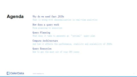
Figure 1: Our Agenda

This won't be super technical, but we'll touch on some technical aspects of how queries run in databases, albeit at a high level. So, it's going to be interesting.

Here's what we'll cover:

1. Understanding Queries: First up, we'll discuss how a query works, from planning to execution.

2. Deep Dive into Query Planning: Next, we'll explore what it takes to generate an optimal or effective query plan.

3. Impact of Computer Architecture: Then, we'll look at how different computing architectures can influence the performance, stability, and scalability of join operations.

4. Exploring Query Execution: We'll also discuss why OLAP databases are generally so fast these days.

Now, let's dive in.

Why Do We Need Joins and Want to Avoid Denormalization?

So, why do we need joins, and why are denormalizations kind of harmful, especially in real-time analytics? When database management systems were invented in the 1970s, it always has been a good practice to keep your data in its most natural and original relational format, like in a multi-table format in Snowflake or a star schema.

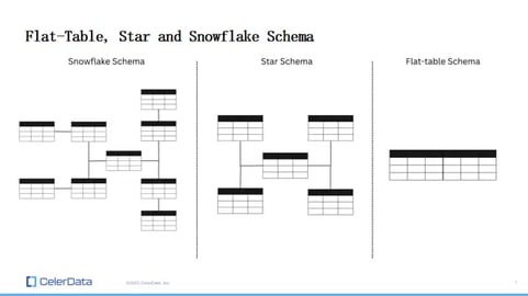
Figure 2: Schema Examples

But it wasn't long until that was no longer the case because many real-time OLAP databases simply didn't handle joins well, or they didn't even have joins in mind when they designed and implemented the system. They actually relied on users to perform a thing called denormalization.

Denormalization essentially means you pre-join your multi-table schema tables, like normalized tables, into a denormalized table, which is a flat table, before the data hits the OLAP database. And that can be quite harmful for several reasons, especially for real-time data analytics.

First, those pipelines are not really that easy to maintain, particularly with the time constraints of real-time. Doing that in batch with Hadoop or with a Spark job, you know, runs for hours, and it might not do a batch job.

It might not be that complicated, but doing that stream, a stateful stream processing job, can be a pain to implement as well as to maintain and configure. It requires additional infra-level software in your data pipeline, as well as much more labor and manpower to actually code and engineering effort to make that happen.

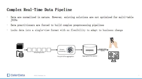
Figure 3: A Complex Real-Time Data Pipeline

The second reason is it really locks your data into a single-view format. So when you do denormalization, you have to know your query pattern beforehand because you're pre-joining everything into one. And it's really difficult to adapt to business changes because it's simple, let's say, changing your data type of a column or adding a column. You have to backfill. You have to reconfigure your entire pipeline and backfill all of your data.

Airbnb case study - moving from Druid to StarRocks

Let's take an example; one of the larger StarRocks users is Airbnb, and they have a Minerva platform that holds around six-plus petabytes of data.

Before, they were using Apache Druid for their query and storage engine. The problem with Druid is that it doesn't handle joins very well, so they had to denormalize everything into big flat tables. And because it's a metrics platform, it stores thousands of metrics.

Changing or adding a metric shouldn't really be a big ask. But with the denormalization pipeline, it becomes a significant ask because reconfiguring the pipeline and backfilling the data can take anywhere from hours to even days, especially considering the scale of data they're operating on, not to mention the additional labor and hardware resources that are being consumed. It's a lot of overhead they're dealing with.

Then they moved to StarRocks because we can perform joins on the fly, so joins are no longer a problem. This way, they can maintain the same data schema in their OLAP database as in their data source.

Benchmark Comparison

This problem is part of the reason we built the StarRocks project. One thing I can count on with StarRocks is that it really handles joins well, probably one of the fastest, if not the fastest, in the market right now. But before we dive into the technical details, let's take a look at some benchmarks.

First, this is an SSB benchmark test, which actually has two variants. There's the original multi-table SSB test, and the folks at ClickHouse created a variant where they denormalized the SSB benchmark into what we call "flat." So it's the SSB without the join part, and join operations are expensive no matter how optimized your engine is.

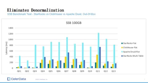
Figure 4: StarRocks, ClickHouse, and Apache Druid Benchmarks

Here, let's look at some results. On the right-hand side, you can see four different colors. Everything with "flat" is run on the variant that is denormalized. The first three, StarRocks is the fastest of all. But the key thing is with the last one; StarRocks multi-table is actually faster than Druid's flat table and almost as fast as ClickHouse flat. This is significant because it alone can indicate that we can really eliminate the whole denormalization pipeline without losing much.

StarRocks is truly an engine or a database designed to scale, especially with complex operations. It performs better than most other solutions, and we're going to delve into the details later.

So this is the SSB benchmark, which resembles more user-facing dashboards or reports, or scenarios where the query is not insanely complex.

Now, let's look at something more extreme, the TPC-DS benchmark test. TPC-DS queries are more complex, resembling ad hoc queries on the data lake and those really intricate ETL queries, your data transformations, and long-running queries.

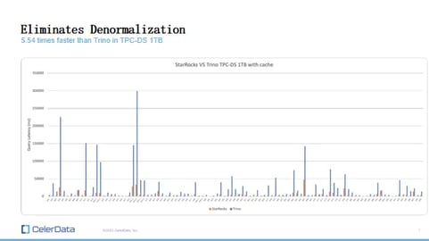
Figure: 5: StarRocks and Trino Benchmarks

We did a comparison with Trino on the TPC-DS 1TB, querying external data as a query engine. StarRocks is 5.54 times faster than Trino on TPC-DS, which is the kind of workload that Trino is best suited for. So, yeah, that's a pretty significant performance increase.

How Does a Query Work?

Yeah, so we talk a lot about the problem and how well we can do it. But how? How do we achieve good multi-table query performance? So, going into that, we need to let's set some foundation, right? Let's take a look at how a query works, from the SQL query to the result. This is really a bird's eye view, and this actually works for most of the databases out there because it's a really high level.

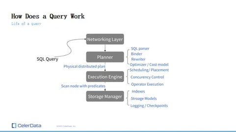
Figure 6: How a Query Works

So you have your SQL query, right, and here's a network layer. The network layer sends the SQL query to your planner, and your planner reads the SQL query and tries to understand it, coming up with a physical distributed plan for our case, right? And the plan is sent to the execution engine, and the execution engine scans the data from the storage engine. Right?

If it's with predicates, hopefully, the predicates can be pushed down, so it doesn't scan all of the data. Right? And that's the capability of your storage engine. It gets the data and, according to the physical plan generated by the planner, the execution engine computes the result and returns that to the user. Right?

Even on a higher level, this is still a multi-layer process, and it requires all of the components to work very well with each other to achieve good scalability, stability, and performance. Right? And on the right, you can see some smaller components of each bigger part, and we're probably going to go into detail with some of them later. Right?

How to generate a good query execution plan?

First, let's delve into query planning and what it entails to generate an effective query execution plan, and how StarRocks handles this. We'll take a closer look at the query plan. This is somewhat like a higher-level flowchart of how a query is planned in StarRocks. This process is pretty generic and similar to how many other databases operate.

So, your SQL query reaches a parser and is converted into an abstract syntax tree (AST). From there, it moves into an analyzer which binds metadata, checks the SQL's legality, and handles aliases.

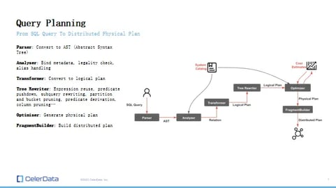
Figure 7: Query Planning

Following this, the query is transformed into a logical plan and is further rewritten to facilitate things like expression reuse, predicate pushdown, among other optimizations. It then proceeds into the optimizer, which generates a physical plan. Subsequently, the fragment builder generates the distributed plan for execution.

An essential point of discussion here is the distinction between a logical plan and a physical plan. The logical plan is more about what the query aims to accomplish, whereas the physical plan is concerned with how it's achieved.

We exert more control during the physical plan stage, highlighting the optimizer as a critical component—one that can make a substantial difference in the entire pipeline.

Query planning - StarRocks' cost-based optimizer

We're going to delve into StarRocks' cost-based optimizer. We have a cost-based optimizer, and optimizing a query is like choosing a route from point A to point B, but the search space is much larger than what you see on Google Maps. The search space of different ways to execute a query is enormous, especially for tasks like join reordering.

The complexity is exponential to the number of tables you're joining together. You have different types of join algorithms and various join strategies on the network level, not to mention some rewrites and many other factors. So the search space is vast. The difference between an optimized plan and an unoptimized plan can be several orders of magnitude.

Sometimes, in the early days, we'd receive an SQL query from a customer where our automation did something nonsensical, and the response time could be minutes. With a simple tweak, that could be reduced to sub-seconds. The disparity is significant, which makes the optimizer an essential part of the infrastructure.

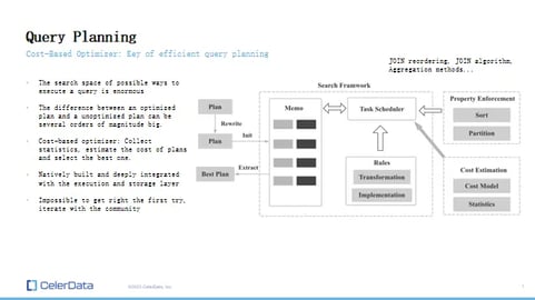
Figure 8: Query Planning Overview

So what does a cost-based optimizer do? Instead of using predefined heuristics and rules to dictate which route to pick, our cost-based optimizer collects statistics and computes the cost of each potential query path or plan, employing a greedy algorithm to select the best one. The statistics collected include aspects like min-max values, the percentage of nulls, the size of the rows, and similar data.

This method has proven to be more efficient, though it's much harder to implement. However, it's a more effective way of generating favorable query plans. It relies heavily on statistics from your storage and the behavior of your execution engine, meaning it's strongly tied to your execution and storage layers. That's why our cost optimizer is natively built and has been refined over a considerable period.

The reality for any optimizer, including a cost-based one, is that it's impossible to get it perfect on the first try. That was true for us as well. For the CBO, our initial release wasn't enabled by default. We underwent an extended period with our seed users where they would report a problematic case, and we'd optimize accordingly.

Our improvements were built on the trials and tribulations of our seed users. But thanks to the community and the fact that we're open source, we've managed to enhance its efficiency to the current level. It wasn't an easy journey, but this is our cost-based optimizer.

Data pruning - global runtime filter

And, another thing I want to touch on is data pruning. This is part of the FE's job as well, and a bit of it is the CBO's responsibility. It's called a global runtime filter. What it does is it minimizes the number of rows or the amount of data the CPU has to deal with during execution. Let's understand this with an example.

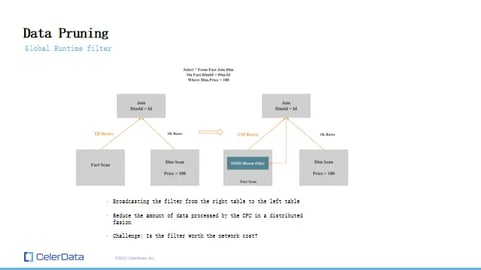
Figure 9: Data Pruning

Okay, so we have a query here: "Select * from fact_table join dimension_table on fact_table.dimension_id = dimension_table.id" Right? And, the predicate is on the join key. And, yeah. The predicate is on the dimension table, and it's "price > 100". Without a runtime filter, how would you run this? The left table, because it has no predicate, you take all of the one billion rows and send that to the join operator. That's what it does.

On the right-hand side, because we have a predicate, it's going to get pushed down to the storage layer. So it's not going to pull all of the data up. It will probably pull up a thousand rows and then do the operation. So what if there's a way we can push this predicate or this where clause to the left table as well? It's probably going to filter out a lot of data.

In this case, let's say it's one billion rows down to a million rows. That's many orders of magnitude less data the CPU has to deal with. This sounds pretty simple, right? In a single-node environment, it's not that complicated because there's no network that's associated with this.

But in a distributed environment, it's very different because we actually have to send this filter to all of the nodes where the other table resides. This incurs a lot of network overhead. So the real challenge is, is the filter worth the network cost? Sometimes it is, sometimes it's not.

This is another CPU story all over again. It needs a lot of optimization. We've had this feature for a pretty long time now, and it works.

Compute Architecture - How Does It Affect JOINs?

Now, let's discuss compute architecture. This is where I see some of the most significant differences between us and many real-time OLAP databases like Clickhouse and Druid, particularly in how we handle join operations. This aspect is crucial in understanding why our joins are scalable.

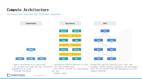
Figure 10: Compute Architectures

Let's examine some different architectures first. I've broadly categorized them into three types at a high level. The first type is scatter-gather. You have a larger task, and you distribute it among various nodes. They each do their part, and the intermediate results are gathered in a larger node, which then returns the result.

This query execution approach can easily bottleneck on a single node because everything converges to one point. It's particularly unsuitable for join operations and high-cardinality aggregations at scale. For instance, in the case of scatter-gather joins, other real-time OLAP databases don't support data shuffling. They rely on other methods more akin to scatter-gather, which can easily create a single bottleneck in the entire cluster. I'll delve into more detail in a couple of slides.

The second type is MapReduce. It's widely used for ETL jobs. You have an operator, and every operator has a map and reduce stage, with all intermediate results persisted to disk. Because everything is saved, it can be incredibly stable. It's not that it doesn't crash, but say you have a task running for five hours and it fails at the third hour.

You can always go back because all the intermediate results are stored on disk, and you can resume your task from the last checkpoint. This is great for long-lasting ETL data transformation workloads. However, it does introduce a lot of performance overhead, making it unsuitable for sub-second or even sub-minute queries. Also, this kind of operation introduces wait times between different tasks.

Then there's the MPP (Massively Parallel Processing) architecture. The most significant difference between MPP and MapReduce is that MPP can operate entirely in memory and supports shuffle operations between the memories of different nodes. Everything runs very quickly, and it genuinely scales.

Because it uses a pipeline execution framework, every time a query hits the database, it creates a sort of DAG or tree-like graph with all the tasks on it, and all the tasks can run simultaneously. This kind of architecture is what StarRocks is based on, and it's excellent for sub-second joins and aggregations at scale.

StarRocks architecture

Taking a higher-level glance at StarRocks architecture, it supports the MySQL protocol from the top down. Hence, you can integrate your preferred BI tools or existing applications, provided they support the MySQL protocol, standard SQL.

Figure 11: StarRocks Architecture

We employ both FE and BE. The FE is akin to the catalog manager, overseeing metadata and query coordination, acting as the query execution pipeline's PM. It determines the query plan the cluster adopts and communicates this to the BE, the execution engine, which can function as a cache or storage engine, handling the heavy lifting.

A primary aspect of StarRocks is MPP. There's a myth to dispel here: MPP doesn't equate to strongly coupled storage and compute. StarRocks indeed advocates a separated storage and compute design from version 3.0 onwards. MPP is truly about parallel processing, offering scalability regardless of workload. Given that we're an OLAP database, we're focused on resolving OLAP queries, especially group by joins, which we can scale effectively.

One pivotal feature of StarRocks is its support for data shuffling, embracing numerous distributed join strategies, details of which I'll delve into shortly. Our capacity for pure in-memory operations renders us highly efficient for low-latency, large-scale join and aggregate queries. The system's performance accelerates with the addition of more nodes.

How To Execute JOINs at Scale

Now, let's dive into how to execute joins at scale, shall we?

It's crucial to recognize that a join operation on a single node contrasts significantly from a distributed join. The latter introduces much more overhead to the entire system, and planning for a distributed join diverges greatly from planning a single-node join. The pivotal aspect we're focusing on here is the join strategy.

This strategy differs from the types of joins we often discuss, such as left join, right join, inner join, or as-of join. It's also distinct from join algorithms like nested loops joins, hash joins, or merge sort joins. We're talking more about the network level here. One of the primary challenges of distributed join operations is disseminating the data to all pertinent workers.

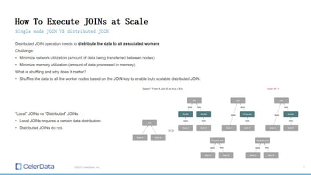
Figure 12: Executing JOINs at Scale

There are a couple of things we're striving to minimize. Firstly, network utilization - we're aiming to reduce the volume of data transferred between nodes. Secondly, we want to cut down the data being processed in memory. It's inefficient to have the same data in the memory of two or more nodes without any performance gain, right?

What is data shuffling and why it matters

So, what exactly is data shuffling, and why is it critical? Data shuffling is the process of distributing all the data to your worker nodes based on the join key. This technique is fundamental to enabling truly scalable distributed joins. I'm going to illustrate this concept with five examples, using two tables for our discussion, which I'll explain sequentially.

Consider table A, which is larger and contains five thousand rows, and table B, a smaller dimension table with a thousand rows. We'll examine various join strategies, what shuffling can provide, and what other options we possess.

I'd like to classify joins into two categories: one being local join and the other distributed join (though I'm not entirely certain if those are the precise terms, they'll suffice for clarity). Local joins necessitate a specific data distribution, so there's no requirement to relocate data during the join operation.

On the other hand, distributed joins don't demand any particular data distribution beforehand, and data is moved around during the join process.

Local JOINs - Collocated JOIN

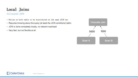
Figure 13: Local JOINs

First up is the collocated join, often referred to as a local join. This method depends on both tables being distributed based on the same join key prior to data ingestion. If that condition is met, there's no need to shuffle any data during the join; each node can independently execute its segment of the join, compile the result, and return it.

This strategy is speedy due to zero network overhead, with everything executed locally. However, it imposes rigidity on the join, reminiscent of the denormalization dilemma. You must be certain of your query requirements in advance and set up everything prior to ingesting the data.

If you need to alter anything, re-ingesting all the data becomes a necessity. While collocated joins are swift, they lack flexibility. They're advantageous if you're confident about the structure of your future queries.

Local JOINs - Replicated JOIN

Figure 14: Replicated JOIN

The second type is another form of local join, known as a replicated join. This method involves replicating the right table to every single node where the left table is located. For instance, if we have three compute nodes, you would have three copies of your right table, let's call it "table B," throughout your entire cluster.

This strategy has the advantage of no network overhead since all of the necessary data is already distributed across all nodes. As a result, the join operation is executed entirely locally. However, the downside is that it consumes a significant amount of storage space because you're essentially storing multiple copies of table B.

Despite this, it's an efficient process and leads to speedy query execution because it eliminates the need for data to be transferred over the network during the join operation.

Distributed JOINs - Broadcast JOIN

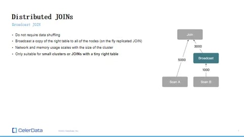
Figure 15: Broadcast JOIN

Next, we're diving into distributed joins. The first one we'll tackle doesn't require data shuffling, but it comes with its own trade-offs. The reason I brought up replicated join is to segue into broadcast join, which you can think of as an on-the-fly, replicated join.

During your query execution, what happens is you broadcast the right table to every node that holds your left table. The number of nodes your setup has plays a big role here.

But here's the snag with this method: the network and memory usage scales not just with the size of your data, but also with the size of your cluster. So, the more extensive your cluster, the more network bandwidth it's going to consume, not to mention the memory usage.

So, it's not really that scalable. It works like a charm for smaller clusters or when the right table is tiny. Have a big fact table and a small dimension table? This will do the job. But if you're dealing with larger tables, especially a larger right table, and this is your only distributed join option, you're going to hit some serious network and memory roadblocks.

Distributed JOINs - Shuffle JOIN

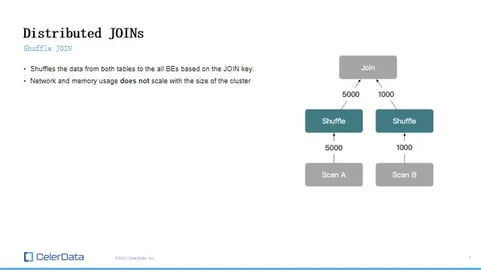
Figure 16: Shuffle JOIN

Now, onto shuffle join. This is something StarRocks leans heavily on for many of its on-the-fly join situations.

Here's how shuffle join plays out: it shuffles the data from both tables to all of the BEs, but it does so based on the join key, and it only does this shuffle once. So, whether your table A has five thousand rows and your table B has one thousand, it doesn't matter how large your cluster is—it's only going to shuffle those rows and spread them evenly, hopefully, across all your BE nodes.

The big takeaway? Network and memory usage doesn't scale with your cluster size, just with your data size. This fact alone makes shuffle join a more scalable solution for join operations when stacked against broadcast join. If your database doesn't support shuffle, well, you're somewhat out of luck.

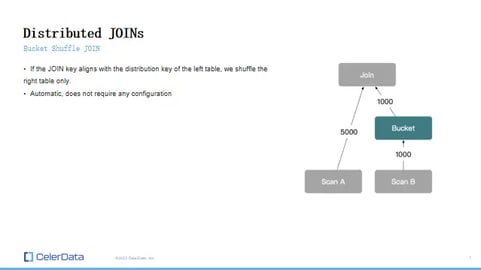
Figure 17: Bucket Shuffle JOIN

There's more to it, though. StarRocks supports variations on this, with one standout being bucket shuffle join. Here, if the join key is the same as the distributed key of the left table, you only have to shuffle the right table. This makes the network cost super affordable, as it's only about the data size of BE, and the same goes for the memory cost.

For this method, memory usage is also only about the size of BE because we can handle it incrementally, downstream.

Recap - built on an architecture that scales

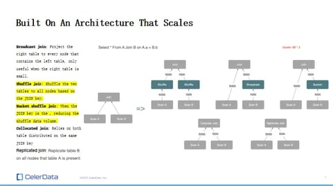
Figure 18: A Strong, Scalable Architecture

Taking a step back, these five methods I've walked through really hammer home how a different compute architecture can make a world of difference. Just by supporting the shuffle operation, you're opening up to a whole range of join strategies on a distributed system, enabling truly scalable join operations.

But this all hinges on your database's ability to handle shuffle operations. Without that, you're either stuck with localized joins where you need to set everything up beforehand or with broadcast joins, which come with a heap of limitations.

Query Execution - How StarRocks Can Use All Your CPUs

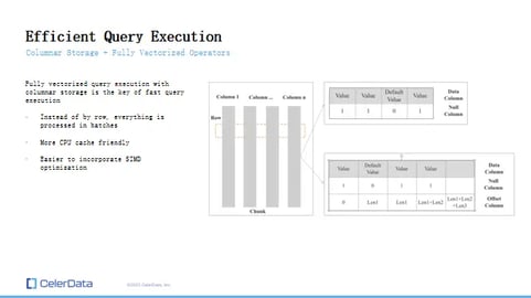
Figure 19: Efficient Query Execution

Let's also touch on query execution because it's a big part of why StarRocks is so fast across the board. It's not just about joins, but the overall speed. StarRocks runs on columnar storage and makes full use of fully vectorized operators.

That means every single operator is vectorized, and in your storage engine, data is stored in columns, not rows. What's vectorized execution? It's when, in memory, you're processing by column, not row. So, for OLAP operations, like joins or group-bys, where you're usually dealing with a big chunk of a column, this method lets us process everything in larger batches.

This makes things more continuous in memory, more CPU cache-friendly, better for CPU branch prediction, and it's especially easy to bring SIMD optimizations into the mix, which we'll get into next.

Efficient query execution - C++ SIMD optimized

StarRocks is constructed using C++, and it's heavily optimized for SIMD (Single Instruction, Multiple Data). To explain, SIMD optimization allows us to process several data points in one go with a single CPU instruction. This means we engage memory far less frequently. Consider the image here, where we have two data vectors.

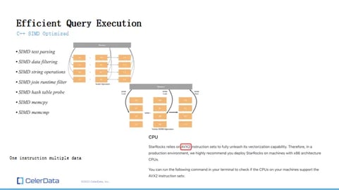
Figure 20: Efficient Query Execution With SIMD

When we execute a vectorized operation, such as multiplication, a scalar operation without SIMD would require fetching and returning data one piece at a time. That's twelve memory accesses and twelve instructions.

However, with SIMD, we need only three because we handle everything in a columnar format and in larger batches. This approach significantly accelerates execution. We've applied SIMD optimization to as many operations as possible, including text parsing, filtering, aggregations, joins, and more.

This optimization is precisely why the AVX2 instruction set is a prerequisite for StarRocks to leverage vectorization capabilities, as it's a SIMD CPU instruction set.

So, that wraps up our high-level explanation of why StarRocks is swift. Of course, there are many more intricacies, particularly during the query planning phase. For instance, how we manage join reordering or how we rewrite subqueries.

Join the StarRocks Slack Channel

If any of this piques your interest, or if there's something specific you'd like to understand better, we invite you to communicate with us on our Slack channel. Join in, and suggest topics for future webinars, or prompt us to write in-depth blog posts that respond to your queries. Also, visit our blog on celerdata.com and consider signing up for the CelerData Cloud at cloud.celerdata.com.

Figure 21: How To Get Involved

Q&A

Let's address some questions now.

Question 1: What steps should I take to optimize queries, or does the query planner handle everything?

Answer: Well, the query optimizer indeed handles a substantial part for you. You don't need to manually sequence the joins or arrange the join tables, for instance — the optimizer takes care of that. Even if your queries are somewhat inefficient, our query optimizer is designed to refine them.

Question 2: Is the 'collect statistic' operation executed in batches, or does it function when cost-based optimization is active? If it's batched, how frequently does it run?

Answer: The process of collecting statistics is automatically handled by StarRocks. If you want to learn the internals of how statistics are collected, you can read the documentation on CBO here.