


Join StarRocks Community on Slack
Connect on SlackWhile normalization stands as a foundational pillar of relational databases, the unsatisfactory JOIN performance of today's real-time OLAP databases has led to a rise in denormalization. This approach, although advantageous in working around the multi-table query performance issues, introduces its own complexities and costs.
-
Rigid Data Pipeline: Denormalization makes the data pipeline less flexible. Any change in the schema might require reconfiguring the entire data pipeline. If historical data needs to be synchronized with the new schema, data backfilling becomes a both time and resource-consuming task
-
Increased Complexity And Cost: In real-time analytics, denormalization necessitates using stream processing tools. This demands not just SQL but actual coding, making the development and maintenance more resource-intensive and costly.
Thankfully, with innovative technologies such as in-memory massively parallel processing, cost-based query planning, and SIMD optimizations, the once-feared on-the-fly JOIN operations have emerged as robust alternatives, mitigating the need for extensive denormalization.
Gone are the days of intricate, maintenance-heavy real-time data pipelines. Today, the most progressive data-driven businesses are going "pipeline-free," and we're here to show you how it's done!
In this engineer-led session you'll learn:
-
New tricks to boost performance and reduce maintenance
-
How to go pipeline-free using only open-source software
-
What does it take to achieve low latency on-the-fly JOINs
-
What businesses like Airbnb are doing to go pipeline-free
-
A technical demo about how global runtime filtering helps with query optimization, data lake analytics, and more
Below is a transcription from the webinar.
Agenda
We're going to discuss real-time analytics. We'll delve into the methodology behind the pipeline-free real-time analytics approach, particularly discussing the issues with denormalization in real-time analytics. We'll then explore how we can achieve pipeline-free real-time analytics and examine the open-source real-time database, StarRocks. I'll also provide a demo on the CelerData cloud, showcasing precisely how a query is planned and executed. It might get technical, but I assure you it'll be engaging.
What is Pipeline-Free Real-Time Analytics?
From the beginning, especially in the 1970s when the database management system was invented, it's been a good practice to keep data in a multi-table schema. This could be in a Snowflake schema, a Star schema, or just considering that data, naturally, is relational.
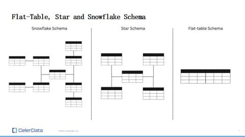
Figure 1: Schema Examples
However, this isn't really the case now, especially for real-time analytics. Many real-time OLAP databases face challenges handling on-the-fly joins with low latency. So, these databases often require users to denormalize their data before ingesting it into the system.
This means everything becomes a single table. Denormalization, in essence, is where you might have data spread across tables, like in a star schema – let's say five tables – and then you pre-join these tables into one flat table, right?
This approach might be fine for batch analytics, where the freshness of insights might vary from a few hours to even days. There, you have the luxury to perform denormalization in batches. But in real-time scenarios, where time is of the essence, it's not quite the same. For real-time, you often need to resort to stream processing tools to achieve denormalization.
What is wrong with denormalization in real-time analytics?
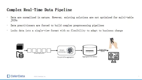
Figure 2: A Complex Real-Time Pipeline
This process can be costly in terms of architecture. You need to maintain a stream processing tool in your real-time data pipeline, which is expensive in its own right. Furthermore, doing denormalization in a streaming fashion, especially when it's stateful, can be technically challenging. It might become unstable and hard to maintain.
Beyond the costs and complexities, denormalization can also lock your data into a specific format. It becomes tricky to change once everything is set. Before setting up the denormalization pipeline, you need to be aware of the query patterns. And once it's configured, making changes to the schema of source tables requires reconfiguring the entire pipeline and backfilling all data.
This is time-consuming, resource-intensive, and expensive. In a business context, small adjustments like changing a column shouldn't be major tasks. But with real-time analytics and denormalization, they become significant operations, right?
So, what's the solution? The key is on-the-fly joins. This challenge with real-time denormalization is a significant reason why we started the StarRocks project. We wanted to address these issues users face. That's why we created StarRocks. Soon, I'll dive deeper into the technical aspects of why StarRocks can handle on-the-fly joins so effectively.
Benchmark test: StarRocks vs. ClickHouse, Apache Druid, and Trino
But in the beginning, I want to show some numbers first. Here, let's first take a look at some benchmark results. This is the SSB Benchmark test. The SSB benchmark test actually has two variants. The first one is the original SSB test which is multi-table. The query test is actually on the fly join. So you're joining everything on the fly.
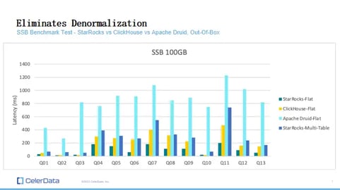
Figure 3: Benchmarks for StarRocks, ClickHouse, and Apache Druid
Then there's ClickHouse. The folks at ClickHouse made another variant where they denormalized the SSB tables. They pre-joined all the SSB tables into one big table and ran all the queries on this single table. That's why on the right side, some are labeled with 'flat' at the end, and others, with 'multi-table' for StarRocks.
Looking at the results, StarRocks is the fastest on the flat schema SSB benchmark test. It's significantly faster than Druid and about twice as fast as ClickHouse. But the crucial thing is the multi-table test. Comparing multi-table results with flat-table ones isn’t really a fair comparison because joins are expensive. Yet, StarRocks' multi-table performance, with the same queries and resources, is better than Druid's single table and almost as good as ClickHouse's single table.
This suggests that StarRocks can reduce the need for denormalization. The performance might be a bit slower, but our architecture ensures that if you add more nodes to the cluster, the query performance scales up, almost linearly. I'll go into the technical architecture discussion soon.
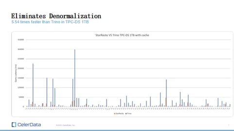
Figure 4: StarRocks and Trino Benchmarks
Because StarRocks has such good query performance, especially for complex OLAP queries, we introduced StarRocks to the Data Lake about a year and a half to two years ago. We also ran the TPC-DS benchmark test. While SSB is more like reports and dashboards, TPC-DS is more complex, like the ad hoc queries data scientists run. It's more challenging than the SSB multi-table schema.
Trino, a well-known open-source query engine for data lakes, is known for its performance. In our tests, StarRocks, querying the same data in the data lake, was about 5.5x faster than Trino, even with more complex queries. I'll discuss how we achieved this in later slides.
Case study: Airbnb
Let's begin by examining some case studies. Specifically, let's delve into Airbnb's Minerva project, a metric management platform. This platform encompasses over seven thousand metrics and stores more than six petabytes of data.
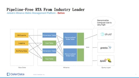
Figure 5: Airbnb's Old Architecture
Prior to their encounter with StarRocks, Airbnb primarily utilized Druid, along with Presto, as their query layer. A significant chunk of their data resided in Druid. The challenge with Druid is its limited capability to handle joins, in many cases not supporting them at all. Consequently, Airbnb found it necessary to denormalize their six petabytes of data, a process that proved to be both time-consuming and costly.
One of the substantial challenges Airbnb faced was the frequent necessity for schema changes. Given the voluminous metrics on the Minerva platform, adjusting a metric was commonplace. However, from a technical standpoint, such changes weren't trivial.
Not only did they have to alter the schema, but they also had to modify the entire denormalization pipeline and backfill data for the flat tables. According to Airbnb, this process could span from several hours to multiple days—a duration that's far from ideal for a company of Airbnb's stature.
In their pursuit of more efficient alternatives, Airbnb pondered the possibility of executing joins on-the-fly. This line of thought led them to StarRocks. Upon integrating StarRocks, they realized that on-the-fly joins were indeed feasible. While they retained some denormalized tables, the majority transitioned to on-the-fly joins.
As mentioned in a webinar Airbnb conducted with us, with StarRocks, denormalization becomes an on-demand process, reserved for exceptionally high-concurrency tasks. By default, all tables remain normalized and consistent with the schema of the original data source.
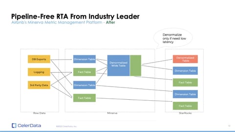
Figure 6: Airbnb's StarRocks-Powered Architecture
This adaptation was monumental for Airbnb. Maintaining a consistent schema between their OLAP database and the original data source significantly streamlined their operations. The need for data backfilling was eradicated.
No longer did they have to configure states for pre-processing or stream-processing jobs. The cumbersome task of reconfiguring pipelines became a thing of the past. Furthermore, all these efficiencies came at a reduced cost and, impressively, with an uptick in performance.
How Do We Go Pipeline Free - A Deeper Look Into StarRocks
How do we attain this remarkable performance on joins, particularly when contrasted with other real-time OLAP databases? In this discussion, we'll delve deeper into StarRocks, the open-source OLAP database. Although things might become technical, I believe it will be an enlightening journey.
Compute architecture: Scatter-Gather, MapReduce and MPP
First, let's take a look at some higher-level compute architecture differences.
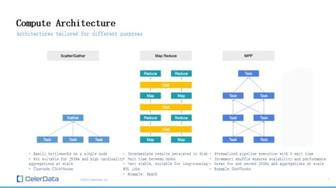
Figure 7: Compute Architecture Examples
-
Scatter-Gather:
-
Overview: In this architecture, tasks are distributed across various nodes. These nodes then return intermediate results to a central node, which carries out the final calculation.
-
Limitation: The architecture can easily experience a bottleneck at a single node. Regarding distributed joins, the main challenge is distributing data across nodes. Most real-time OLAP databases with this model don’t support the shuffle operation, so they rely on broadcast joins. This involves broadcasting a smaller table to all larger tables. This method doesn’t scale efficiently; as the cluster size increases, so does memory usage. Hence, it's not a truly scalable solution for distributed joins.
-
-
MapReduce:
-
Examples: Systems such as Hadoop and Spark use this approach.
-
Overview: In this model, operators perform both map and reduce functions. All intermediate results are stored to disk.
-
Pros & Cons: Although it supports data shuffling, writing intermediate results to disk can lead to unsatisfactory low-latency performance. This architecture is suitable for ETL jobs due to disk persistence, providing good fault tolerance. In case of a query failure, the system can revert to the last checkpoint. However, it's not the best fit for low latency querying.
-
-
Pure In-Memory MPP (Massively Parallel Processing) Architecture:
-
Overview: This is what StarRocks uses. It streamlines the query execution process, ensuring minimal wait times between tasks as nothing gets persisted to the disk. Moreover, it facilitates in-memory data shuffling, allowing nodes to communicate via shuffle tasks.
-
Advantage: This approach is the main reason StarRocks can efficiently handle high-performance, scalable joins on a large scale.
-
This gives a glimpse into the architectural considerations of StarRocks and how it differentiates from other architectures.
Query planning - cost-based optimizer
Let's delve into the process of executing a query. At its core, running a query is fundamentally a two-phase process.
-
Query Planning: This is where you interpret the query's intention and develop a plan. That plan is then sent to the compute nodes for actual execution. The significance of query planning can't be overstated. An optimized query plan and an unoptimized one can have differences that span several orders of magnitude.
I've seen scenarios where, due to suboptimal planning, the execution discrepancy reached thousands of times. This step involves intricate decisions such as choosing join strategies, determining join ordering, and selecting aggregation methods. The potential ways to execute a query, especially an OLAP one, are vast. For instance, deciding on join ordering alone is an NP-hard problem.
-
Execution: Here, the compute nodes execute the query and return the result.
Given the complexities in query planning, we invested a lot in building our cost-based optimizer. This optimizer collects data statistics and uses this information to estimate the cost of each potential plan, eventually selecting the most efficient one. While this may sound straightforward, it's not. The process requires in-depth optimization.
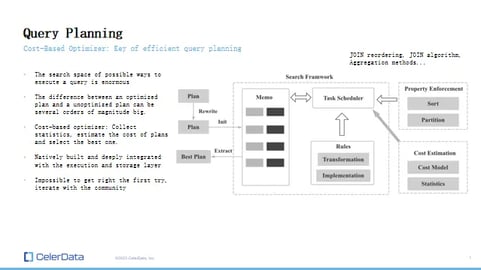
Figure 8: Query Planning
StarRocks' cost-based optimizer was built in-house because an effective optimizer should be deeply integrated with the execution and storage layers. It's not about merely adding an open-source optimizer to a database and expecting peak performance.
Our journey with the StarRocks cost-based optimizer has been a long one. Initially, when released, it wasn't even active by default. We collaborated with our early users for nearly a year to refine its performance. This rigorous development process is a key reason why StarRocks excels at on-the-fly joins.
Query execution - columnar storage + fully vectorized operators
Let's take a look at query execution. StarRocks features a combination of columnar storage and fully vectorized operators. This design isn't only for handling joins but serves as the main reason StarRocks is fast, not just for joins but for large-scale aggregations and other types of queries as well.
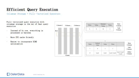
Figure 9: Efficient Query Execution
Columnar storage means data is stored by columns rather than rows. And when we talk about vectorized operations, it means that everything is processed by columns when in memory.
This approach is highly efficient for OLAP workloads because they typically process data by columns. Processing everything by column allows us to handle larger batches, which makes it much more feasible to implement SIMD optimizations. I'll discuss this in more detail in the next slide.
Query execution - C++ SIMD optimized
StarRocks stands out because our execution engine is built entirely in C++. This foundation allows us to leverage a broad range of instruction sets to boost our query speeds.
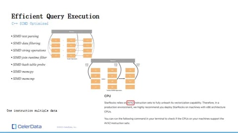
Figure 10: SIMD Optimization
So, what does SIMD mean in the context of databases? Essentially, SIMD allows for the processing of multiple data points using a single instruction, minimizing memory seeks in the process. If you think of a scalar operation, it's a bit like having two vectors, performing an addition operation on them, and then getting another vector as a result. In this process, you have to access memory multiple times. However, with SIMD addition, the number of times you need to access memory is greatly reduced, speeding up the entire operation.
In StarRocks' query engine, we've ensured that as many operations as possible are SIMD optimized. Currently, almost all of them have been optimized in this manner, whether it's filtering, parsing, joins, aggregations, or other operations. This focus on optimization is why StarRocks mandates the use of the AVX2 instruction set, a specific type of SIMD instruction.
Partial update for high-concurrency scenarios
Regarding on-the-fly joins, as efficient as they might be, they're still quite resource-intensive. Regardless of how well you've optimized your query layer, joins remain costly operations. When dealing with customers who have tens of thousands of QPS, executing on-the-fly joins isn't always feasible, even with a robust database like StarRocks. So, what's the solution?
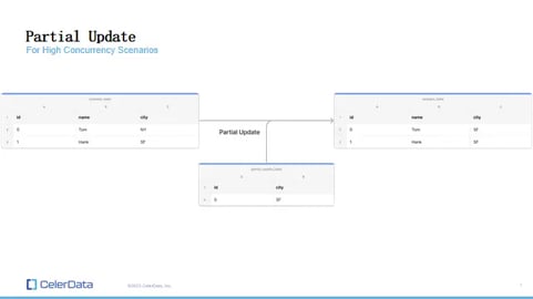
Figure 11: Partial Updates
The approach we've taken is straightforward. Instead of relying on denormalization via pre-processing or streaming tools, we offer the capability for partial updates directly within the columnar storage.
In practice, this means you could have one data stream, perhaps sourced from Kafka, and another separate data stream. Both of these streams can concurrently perform data upserts to the same table. This method facilitates denormalization within the database itself, eliminating the need for extensive computation or external processing tools.
While this sounds simple, implementing it was quite challenging. It necessitated various optimizations, but it's a feature we've dedicated significant time to develop. Our aim is to allow our users to operate without the need for additional pipelines and to bypass any preliminary denormalization.
Demo: A Look at CelerData Cloud
I represent CelerData, and we are the maintainers of the StarRocks project, specifically the StarRocks open-source project. We offer a cloud solution for StarRocks named CelerData Cloud. CelerData Cloud is built entirely on StarRocks, delivering the same excellent performance, but also managing the maintenance tasks on your behalf.
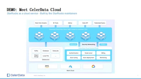
Figure 12: CelerData Cloud Overview
Its operation model is BYOC – Bring Your Own Cloud. Instead of deploying the database in our VPC, we deploy it within your VPC. However, we do have a management service in our VPC that assists with database management and related tasks. Additionally, there's an SQL editor I'll introduce shortly.
We adopt this model to ensure the highest level of security for you. You maintain control over your deployment and all your data. Now, let's move on to a demonstration where I’ll present what the cloud interface looks like. You should now be viewing my screen displaying the CelerData Cloud in a Chrome window.
This is the CelerData Cloud BYOC interface, where I already have a cluster established. This was set up last week and operates on version 3.0.3 of StarRocks. The cluster comprises one FE node, responsible for query planning and the cost-based optimizer. Despite its modest size, with only three nodes and four extra-large MCI, it functions seamlessly.
Demo: CelerData Cloud - capabilities
CelerData Cloud's operational model follows the BYOC (Bring Your Own Cloud) approach. Rather than deploying the database within our VPC (Virtual Private Cloud), it is set up within your VPC. Concurrently, we have a management service in our VPC that oversees database management and related operations.
Furthermore, we have incorporated an SQL editor, which I'll demonstrate shortly.
Our primary motivation for adopting this model is to ensure utmost security for our users. With this setup, you retain control over your deployment and, by extension, all your data. Now, I'd like to walk you through a brief demo to give you a visual idea of what our cloud interface looks like. Let me share my screen.
Can everyone view my screen? You should be seeing a window titled 'CelerData Cloud' on Chrome.
As you can observe, this is our CelerData Cloud BYOC interface. Currently displayed is a cluster I set up last week for a demonstration. It's running on version 3.0.3, which corresponds to the StarRocks version.
At the heart of this system is StarRocks, functioning in the background. The details of the cluster highlight a single FE node. This FE node, a critical component of CelerData, handles crucial tasks such as query planning. It's integral to the cost-based optimizer we discussed previously. Observing the node type, our cluster is relatively compact, consisting of just three nodes equipped with four extra-large MCI.
Demo: CelerData Cloud - query planning and execution - global runtime filter
Let's dive in. Alright, as we enter the interface, you'll notice I have a database named TPC-DS one terabyte. Prior to this webinar, I contemplated how best to demonstrate the join capabilities of StarRocks. One approach would be to simply load the TPC-DS one terabyte dataset and run the query live. But having already showcased the benchmark, that approach seems redundant.
Here's where it gets interesting. Consider running a complex OLAP query. A primary goal in such cases is to minimize the volume of data the CPU processes. While many databases can accomplish predicate pushdown – pushing a WHERE clause down to the storage layer so that not all data is scanned – this process varies greatly in its efficiency and effectiveness across different scenarios.
This brings us to an impressive feature of StarRocks: the Global Runtime Filter. I'll demonstrate this using the TPC-DS benchmark test. The purpose here is to provide insights into how queries are planned and executed within our console.
To start, I've selected four tables relevant to our demonstration:
-
Store Sales: The largest table in TPC-DS for one terabyte, boasting a staggering 2.87998 billion rows.
-
Customer: This table holds around twelve million rows.
-
Item: A relatively smaller table with three hundred thousand rows.
-
Call Center: The smallest table, containing just forty-two rows.
Let's dive deeper into these queries. For the first one, we are joining the substantial store sales table with another table using a join key. Furthermore, the predicate in this query is also the join key, present in both tables.
At first glance, it may seem straightforward. However, examining the query profile, it's evident that StarRocks pushes the predicate of the customer table to the other table, minimizing the data scanned.
This approach is efficient when the predicate column exists in both tables. But what if the predicate is unique to just one table? Filtering data from a larger table based on a predicate from a smaller table without the said predicate can be challenging. Yet, our Global Runtime Filter shines in this aspect.
When we run the query, despite the absence of the predicate in the store sales table, StarRocks recognizes and eliminates this from the query execution, thus reducing the processed data.
A detailed look at the query profile reveals that even though all data is scanned, the runtime filter dramatically reduces the data processed during query execution. This optimization allows the query to run in mere seconds, an impressive feat given the vast amount of data and the compactness of our cluster.
StarRocks' optimizer dynamically decides the efficiency of pushing a predicate to the storage layer. If the predicate result set is large, it might not deem it worthy of being pushed down.
However, when working with smaller result sets, like from smaller tables, the predicate does get pushed to the storage layer. This adaptability underscores the intelligence of our query planning, shifting strategies based on the data at hand – a true embodiment of a cost-based approach to query optimization.
In conclusion, while StarRocks' storage engine is innately fast, it's our exceptional query planning and features like the Global Runtime Filter that make it a standout. If you have any questions or need clarification on any point, please don't hesitate to ask.
Demo: CelerData Cloud - data lake: data catalog
Indeed, we've brought that same level of performance to the Data Lake. One of the features StarRocks offers is the "data catalog". Essentially, a catalog functions as a metadata manager. By default, StarRocks comes equipped with its own metadata management tool, known as the internal catalog.
Additionally, users have the option to incorporate external catalogs, facilitating connections to various data lakes like Apache Hive, Iceberg, Hudi, Delta Lake, and we also support Paimon, among others.
Now, let's explore connecting to AWS Glue, specifically with data stored on S3. For demonstration purposes, we'll name this connection "Glue Catalog", and I'll specify the region where my data resides, which is Oregon, US West. Consistently, our AWS Glue region remains in Oregon. An added advantage when using Glue is that the default format is the Hive table format. Once this setup is complete, the following steps are fairly straightforward.
Having already set the necessary parameters, we'll opt for profile-based authorization to establish our catalog. Upon completing this action, you've essentially gained access to data on your data lake, which in this scenario is housed on an S3 bucket, with metadata oversight provided by AWS Glue.
From here, we can inspect the available tables sourced from the Parquet file. A cursory glance reveals the tables from our newly created Glue Catalog. These tables were added with just a few uncomplicated steps. Furthermore, if desired, we can designate this as our default database.
Let's try out a simple query, say, counting the number of store sales. What's happening behind the scenes is that we are directly fetching data stored on S3. This table might seem familiar, yet the data source is entirely different, given its placement on the data lake.
It's worth noting that StarRocks isn't confined to real-time analytics; while it boasts a robust storage engine with real-time capabilities, it can also serve as a high-performance query layer on a data lake. In this capacity, it outperforms many other market solutions.
Concluding my demonstration on CelerData cloud BYOC, I genuinely hope you found it informative. While we're still connected, I'd love to share a few additional insights.
Get Started With StarRocks and CelerData
And so this is the StarRocks project. Please take a moment to explore it. We've garnered 5.3k stars - and we'd appreciate if you could give us a star as well! The project is open source and entirely free. This means you're welcome to review the source code, download the binary, and test it out on your own.
If you're looking to quickly dive in, starting is straightforward. Just use a simple 'docker run' command, and you'll be up and running, experiencing our exceptional join performance. Additionally, for a wealth of information, you can visit our website at CelerData.com.
Our blog section offers numerous articles that delve into topics like user-facing analytics, data lake management, real-time analytics, and strategies to reduce costs associated with real-time analytics. It's a valuable resource worth checking out.
With that, I believe I've covered the primary points. I'll now stop sharing my screen. Thank you so much for your attention during this demo.
For further exploration, here are some resources you might find beneficial:
-
Sign Up for CelerData Cloud: Register today and enjoy a 30-day free trial.
-
Connect with our Community: Join our Slack channel.
That sums up everything from my end. Thank you!
Q&A
Now, let's answer some questions.
Question: How Does Real-Time Analysis Impact Decision Making And Operational Efficiency
Answer: Yeah, so, for real-time analytics, it's really dependent on your use case. Right? If you're tackling something like fraud detection, having data available in real time and the capability to query it within seconds is crucial. You're aiming to catch fraud in real time, right? So, the most suitable approach is to analyze your own use case.
Even though the cost of real-time has decreased significantly over the years due to newer solutions, there's still some overhead with real-time analytics. You'll often need different tools and practices. So, before jumping into real-time analytics, ask yourself if your situation truly benefits from it. It varies for each business.
Question: What Are The Reasons That StarRocks Is Faster Than Trino?
Answer: Trino can handle joins quite well, but StarRocks has its advantages. One primary reason is that StarRocks is built on C++, while Trino is Java-based. This allows StarRocks to utilize SIMD instructions, which can be very beneficial for large-scale OLAP queries and complex operations. This is mainly the reason for the difference in speed.
Question: Can StarRocks Perform Real-Time Update?
Answer: Yes, StarRocks does support this. It features a primary key index. While many solutions in the industry employ a merge-on-read approach for data updates, which can negatively impact query performance, StarRocks uses a merge-on-write strategy. This means data updates are handled during ingestion without compromising query performance. So yes, it natively supports data updates, and with its unique storage engine, it can handle frequent updates at high volumes.
Question: What Data Lake Does StarRocks Support as a Query Engine?
Answer: StarRocks currently supports Apache Hive, Apache Iceberg, Delta Lake, Hudi, and Paimon. Those are the primary data lake table formats it can work with.
It seems we've addressed the attendee questions for now. If there are more questions from the audience, we're here to answer them.
Go Pipeline-Free With Real-Time Analytics
Lastly, if there's one central message I'd want our audience to retain today, it's the concept of going pipeline-free. If you're contemplating using real-time analytics, understand that denormalization isn't an unavoidable obstacle. Innovative solutions, including StarRocks and a few others, can efficiently handle joins on the fly, eliminating the need for denormalization.