


Join StarRocks Community on Slack
Connect on Slack*The content of this blog post is based on our recent webinar, "From Denormalization to Joins: Why ClickHouse Cannot Keep Up".
ClickHouse has long been praised for its performance, but that performance is limited to the local maximum offered by solutions dependent on denormalization. Significant advances in JOIN technology now allow you to ditch denormalization and enjoy record-setting performance improvements in return. Learn all about those advances and how you can break free from the limitations of denormalization.
Intro & Agenda
Let's begin. Today's topic is "From Denormalization to Joins: Why ClickHouse Cannot Keep Up." I'm Sida Shen. Welcome, everyone.
Today, we'll discuss:
-
Data modeling and denormalization.
-
Why on-the-fly joins are superior to denormalization.
-
Case studies from industry leaders like Airbnb, highlight their move away from denormalization to a more streamlined analytics pipeline.
-
Technical aspects of why ClickHouse struggles with on-the-fly joins.
-
A high-level comparison between ClickHouse and other open-source solutions in terms of query planning, distributed compute architecture, and query execution.
Data Modeling Best Practices - Normalization vs. Denormalization
When we think about data modeling, three main schemas come to mind: flat table schema, star schema, and snowflake schema. While flat table schema consolidates everything into one table, star and snowflake schemas are multi-table, relational systems.
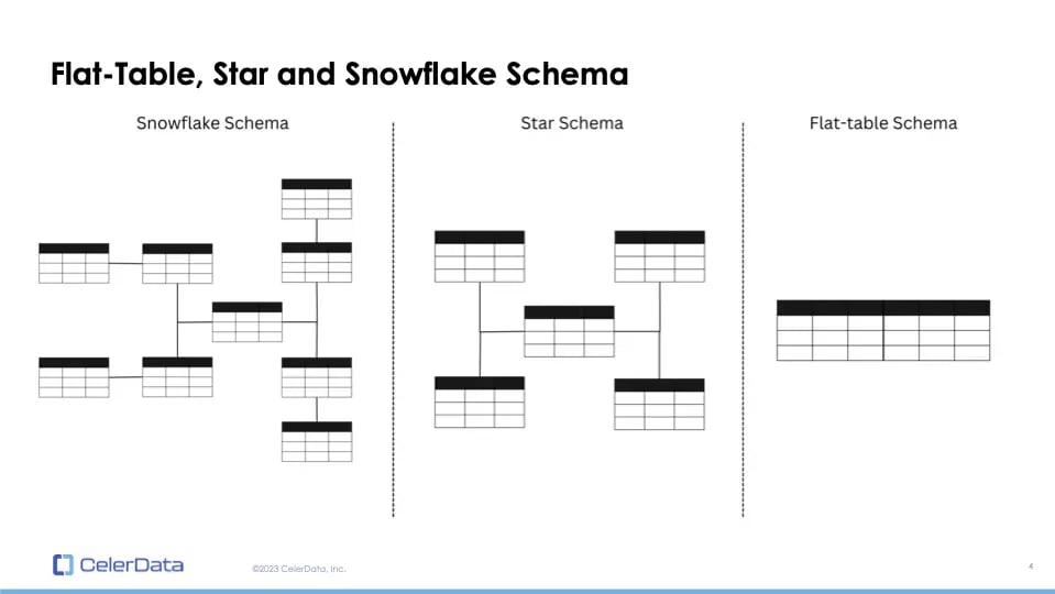 Figure 1: Data Modeling
Let's discuss data modeling and the various types of data models available. These include flat table schema, star schema, and snowflake schema.
A flat table schema consists of a single table where all data is stored in one large table. On the other hand, star and snowflake schemas are multi-table models. They're relational, meaning multiple tables relate to each other based on certain columns or keys.
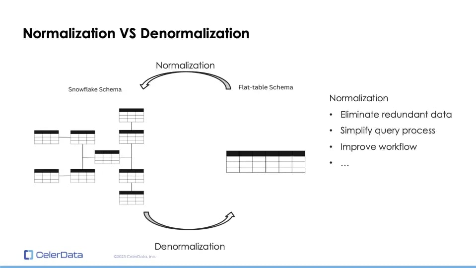 Figure 2: Normalization vs. Denormalization
Normalization involves converting a flat table schema to a snowflake schema, and denormalization is the reverse process. Normalization has been a best practice for database management systems since the inception of relational databases, nearly fifty years ago. This approach eliminates redundant data, simplifies query processes, and overall improves workflows.
Why Denormalization Is Harmful
However, with Online Analytical Processing (OLAP), particularly in real-time analytics, denormalization has become more common. This is because join operations are expensive and many database vendors choose not to optimize them. Instead, they rely on users to denormalize their data to avoid joins. This practice can be problematic.
Complex real-time data pipeline
Consider this example: On the left, we have a customer table, and on the right, an order table. Both tables contain a 'customer ID' that serves as the JOIN key. Suppose a data engineer wishes to create a dashboard without performing a join operation due to database limitations. The engineer might denormalize the tables into a single, flat table based on the 'customer ID'.
However, if a requirement arises to mask customer names for security reasons, it introduces complications. The data engineer would have to modify the source tables, reconfigure the data pipeline, and backfill the entire 'customer name' column on the flat table. A seemingly simple change becomes quite complicated due to denormalization.
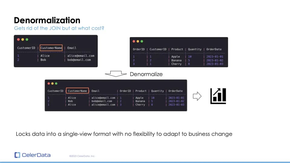 Figure 3: Denormalization
Denormalization essentially locks data into a single view, reducing flexibility to adapt to business changes. Consider the scale: even if the customer table has hundreds of thousands of entries, the order table could have billions. Backfilling such extensive data is more costly than it appears at first glance.
Complex data pipeline
Denormalization makes analytics rigid and less adaptable to business changes. Moreover, it adds complexity, especially in real-time data analytics.
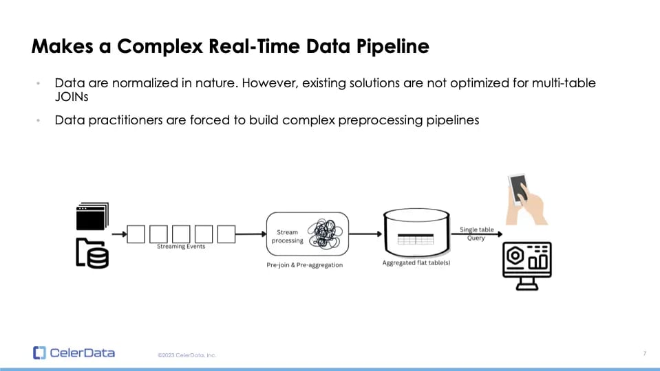 Figure 4: Complex Real-Time Analytics Data Pipeline
In real-time scenarios, batch analytics tools like Spark may not be suitable. Instead, stateful stream processing tools are needed, which are known to be challenging, and require significant technical expertise. Many of these tools don't even fully support SQL, necessitating actual code for efficient usage. In essence, denormalization significantly increases the complexity and cost of real-time data pipelines.
The Solution To the Denormalization Problem - On-the-fly JOINs
The solution? Speed up JOIN operations so denormalization becomes unnecessary.
Introducing StarRocks
This brings me to StarRocks, the real-time OLAP database. StarRocks is cloud-native, storage and compute-separated, and supports real-time mutable data with no external dependencies. It's also Standard SQL-compliant.
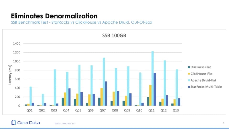 Figure 5: StarRocks, ClickHouse, and Apache Druid Benchmarks
Its strongest feature? Efficient JOIN queries. In benchmarks, StarRocks consistently outperforms other databases, even when handling multi-table JOINs. In the SSB benchmark test, StarRocks' performance on the SSB flat dataset outperforms StarRocks' multi-table performance and even outperforms Apache Druid's single-table performance and almost as fast as ClickHouse's single-table performance.
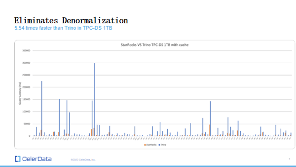 Figure 6: StarRocks vs. Trino Benchmarks
Airbnb case study
To illustrate, let's look at Minerva, Airbnb's metric platform. Initially, they relied on Apache Druid and Presto, requiring extensive denormalization. This process was storage-intensive and cumbersome. But with StarRocks, they found a more efficient and streamlined approach.
A significant change is the shift from default denormalization to on-demand normalization. Currently, only about 20% of the tables are denormalized for high concurrency or very low latency, while the majority are normalized. This transition has resulted in considerable time and monetary savings.
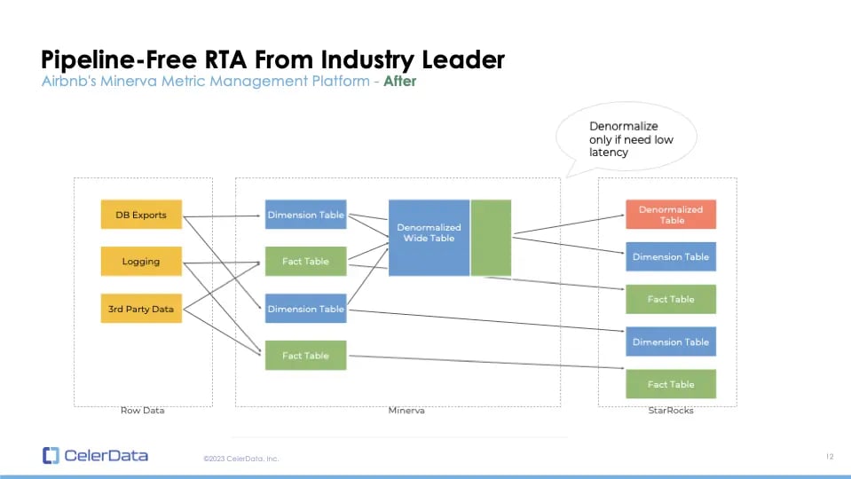 Figure 7: Airbnb's StarRocks Solution
Tencent Games case study
I also want to discuss Tencent Games. Previously, they utilized technologies such as PostgreSQL and MySQL. These systems couldn't perform joins or on-the-fly aggregations, necessitating pre-computed joins and aggregations. This approach posed a challenge since any analytical task required the creation of a separate pipeline, hindering multidimensional self-service analytics. Furthermore, they faced difficulties in maintaining two distinct pipelines for real-time and batch operations, a complex and costly endeavor.
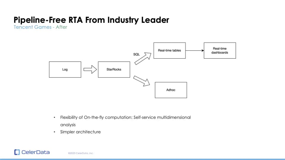 Figure 8: Tencent's StarRocks Solution
After transitioning to StarRocks, they were able to consolidate their operations. StarRocks not only facilitates swift on-the-fly aggregations but also supports on-the-fly joins. This means there's no waiting for pipelines or pre-aggregations, allowing analysts to perform multidimensional analytics more efficiently. The shift to StarRocks has also led to a simplified architecture.
Technical Comparison Between ClickHouse and StarRocks
While systems like ClickHouse can't perform JOINs, StarRocks can. This distinction leads us to discuss the technical aspects of how a query operates.
How does a query work?
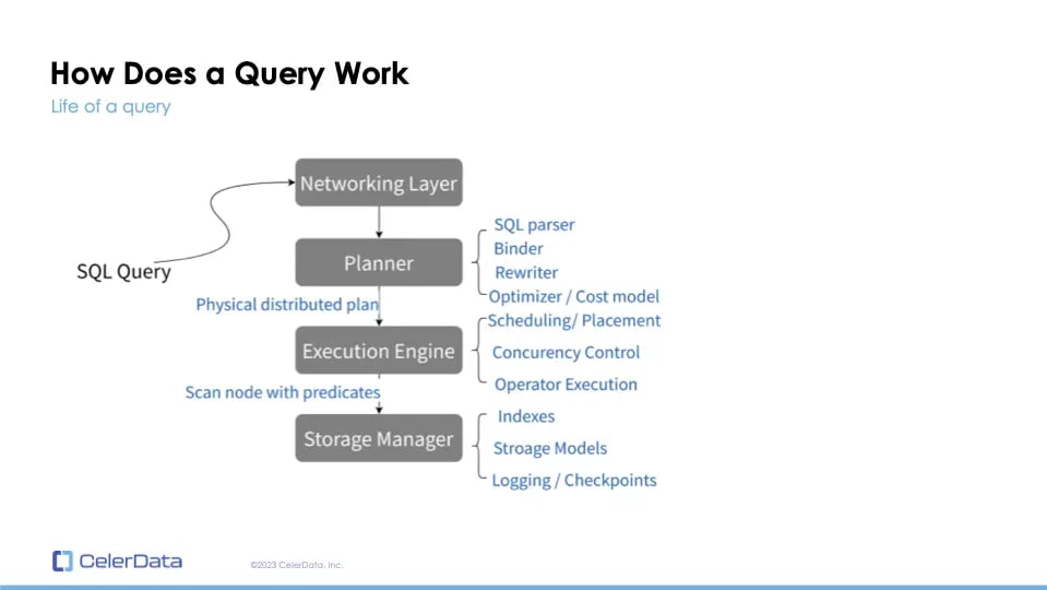 Figure 9: How a Query Works
Two vital components in this process are the planner and the execution engine. The planner's efficiency in devising a route is crucial, irrespective of the execution engine's speed. If the plan is not optimal, achieving a low query latency becomes impossible. The execution engine's architecture should ideally utilize all the CPU cores across the cluster, ensuring optimal performance. Let's delve deeper into query planning and understand what makes an efficient query execution plan.
Query Planning
Let's delve into the intricacies of query planning. When an SQL query is executed, it first encounters the parser which generates a syntax tree. This tree then undergoes a transformation process to produce a logical plan. The optimizer takes this logical plan and generates a physical plan, where the real optimization occurs. While the logical plan represents the intent of your SQL, the physical plan dictates how the database will execute this query, whether on a single node or across a distributed system.
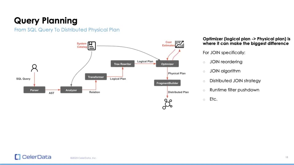 Figure 10: Query Planning
The optimizer plays a pivotal role in ensuring swift queries. Consider joins; there are multiple methods to execute them, involving the reordering of tables and the selection of varying join algorithms and strategies. Advanced features, such as runtime filter pushdowns, add complexity. The distinction between an optimized and unoptimized plan can be vast, sometimes differing by several orders of magnitude.
Differences between ClickHouse and StarRocks' optimizer
ClickHouse employs a rule-based optimizer, which decides based on a predefined set of rules or heuristics. It has limited regard for actual data distribution, focusing mainly on basic metrics like file size or row count. Rule-based optimizers can suffice for uncomplicated queries, but they might not be ideal for OLAP workloads.
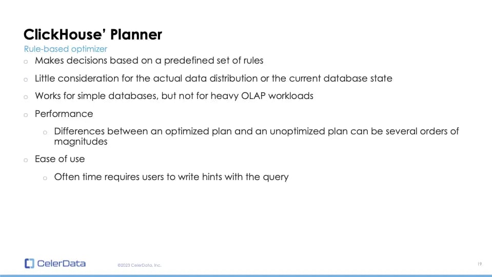 Figure 11: ClickHouse Planner Overview
In contrast, StarRocks utilizes a cost-based optimizer that gathers statistics, estimates plan costs, and applies a greedy algorithm to select the most efficient plan. This optimizer is an intrinsic part of StarRocks, deeply integrated with its execution and storage layers. Optimizer development is a complex endeavor, demanding multiple iterations, especially in open-source projects like StarRocks.
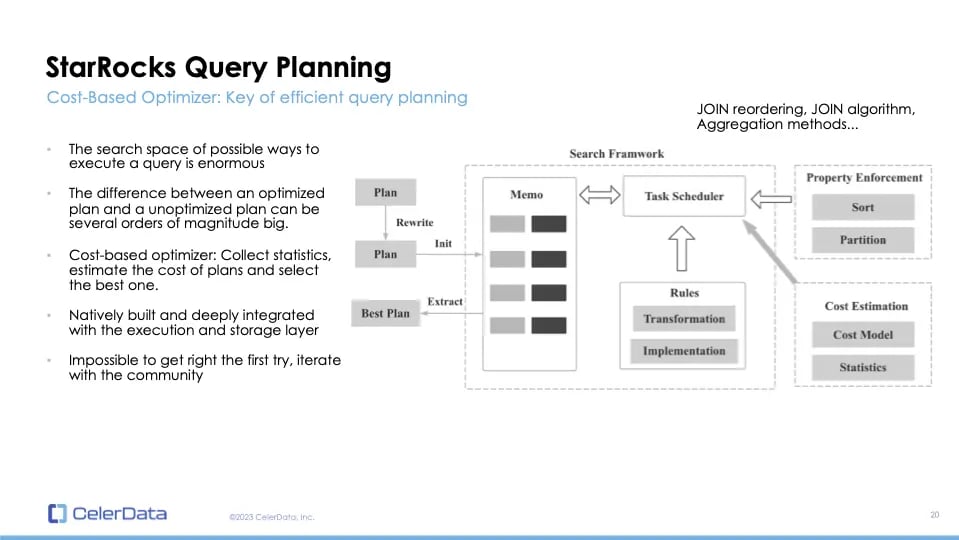 Figure 12: StarRocks Query Planner
Beyond the optimizer, StarRocks has implemented numerous other optimizations to minimize CPU data processing. One such method, the global runtime filter, involves transmitting a bloom filter between tables during queries, ensuring only necessary data is being processed. You can watch the demo here.
Compute Architecture - How Does It Affect JOINs?
The architecture of computing also heavily influences join operations.
JOIN related concepts
There are various join types—inner, outer, cross, semi, etc.—that depict a user's intent. Then, there are join algorithms, like hash join or merge sort join, determining how a join is executed on a single node. Finally, join strategies—such as local, co-located, or broadcast joins—determine the approach for distributed joins.
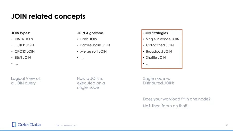 Figure 13: JOIN Concepts
An essential question arises: Can your OLAP workload be managed by a single node? Given that joins are among the most resource-intensive operations in SQL, if the answer is "no", focus shifts to join strategies.
Shuffling: The answer to the scalable JOIN challenge
The challenge of distributed joins lies in ensuring every worker node receives the right data while minimizing network and memory utilization.
You don't want the same data being copied everywhere without achieving multiple conformances. Let me introduce the concept of data shuffling.
Why does shuffling matter for join operations? Data shuffling is the act of redistributing data to worker nodes based on a join key. By shuffling the data, either from the left or the right table, we ensure a truly scalable distributed join. I'll demonstrate this with examples like shuffle join, broadcast join, bucket shuffle join, and localized or single node joins.
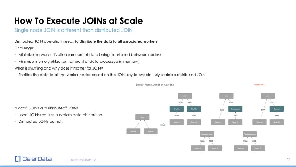 Figure 14: Executing JOINs at Scale
Let's first discuss different join strategies. The first type is the local join, which I refer to as a single node join. Using multiple nodes for a query with a local join requires specific data distribution. You need to pre-organize your data for the join to be executed across multiple nodes. In contrast, distributed joins send data on-the-fly during query execution.
First, consider the local join, specifically the co-located join. This join type doesn't send data. Instead, it relies on both tables being distributed on the same join key. To utilize co-located join, one needs to be aware of the join condition beforehand. The join is executed locally, eliminating network overhead, making it fast but less flexible. You need prior knowledge of the query before ingesting the data, and no data shuffling is required.
The second type is a distributed join known as broadcast join. This join doesn't require data shuffling but has limitations. For instance, if you have a larger left table and a smaller right table, the smaller table is broadcasted to all worker nodes.
Assuming we have three nodes and the right table has a thousand rows, the network overhead becomes three thousand rows. It's expensive, and the right table must fit into every worker node memory. This approach suits smaller clusters or joins with a minimal right table. Notably, ClickHouse can only support this type of distributed join due to its lack of data shuffling capabilities.
Next is shuffle join. It distributes data from both tables to all nodes based on the join key. It's highly scalable: as you add more nodes, performance increases without demanding more memory for the same query. This method is crucial for achieving truly scalable joins in a distributed setting.
StarRocks has optimizations like the bucket shuffle join. If the join key matches the distributed key of the left table, only the right table is shuffled, reducing network load. This process is automatic and configuration-free. The ability to shuffle data is essential.
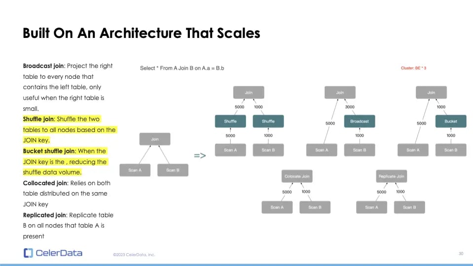 Figure 15: A Scalable Architecture
We covered broadcast join, shuffle join, bucket shuffle join, co-located join, and replicated join. Replicated join, a precomputed broadcast join, duplicates the right table onto every node during data ingestion, utilizing storage. Without shuffling capabilities, ClickHouse's only options are to either predetermine your query pattern and distribute data accordingly for co-located or replicated joins or use broadcast join for smaller right tables. In scenarios where both tables are vast, shuffling is imperative, lest you experience bottlenecks from single node limitations.
Compute Architecture - Scatter/Gather, Map Reduce and MPP
Now, let's delve into compute architecture. We've discussed how a query is executed, both on a single node and in a distributed manner.
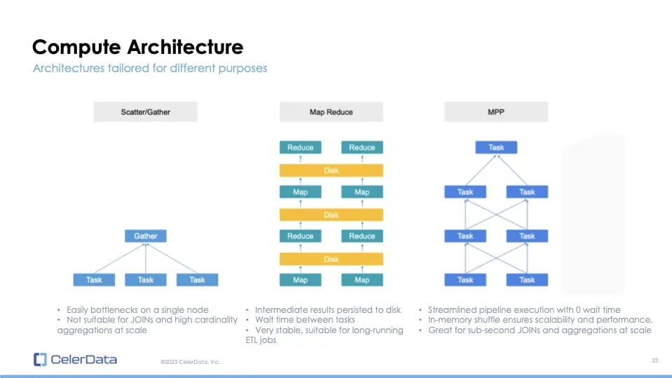 Figure 16: Compute Architecture Example
The first type of compute architecture is the scatter-gather method. Here, a leader node distributes tasks to follower nodes. These follower nodes compute and send aggregated results back to the leader node for the final calculation. This is the model that ClickHouse uses, and it's prone to bottlenecks on a single node.
Next, we have the stage-by-stage or map-reduce architecture. This supports data shuffling, allowing for computations between shuffles. However, each shuffle and the associated map and reduce processes must be persisted on disk. This architecture is stable and suitable for long-running ETL jobs but isn't optimal for low-latency queries. For example, Spark and its photon engine by Databricks use this architecture.
Then we have the pure in-memory MPPs. This supports data shuffling between the memory of worker nodes, ensuring minimal wait times. It's efficient for quick joins and high-cardinality aggregations.
Regarding StarRocks' architecture, it adopts a storage and compute separation. A misconception I'd like to address is that MPP implies coupled storage and computing. In reality, MPP means data shuffling ability and scalable workload with additional nodes. It doesn't imply combined storage and computing.
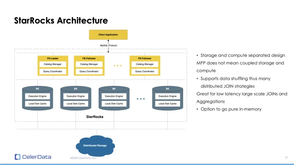 Figure 17: StarRocks Architecture
With its support for data shuffling and diverse join strategies, StarRocks is excellent for low latency, large-scale joins and aggregations. It also offers a pure in-memory option for faster queries.
 Figure 18: Connect With Us
Conclusion & Takeaways
To conclude, let's compare StarRocks and ClickHouse:
-
StarRocks supports on-the-fly joins, while ClickHouse requires complex denormalization data pipelines.
-
For query planning, StarRocks uses a cost-based optimizer, whereas ClickHouse relies on a rule-based optimizer.
-
StarRocks has further optimizations for joins, such as the global runtime filter. To learn more about this filter, you can watch a demo on the CelerData YouTube channel.
-
In terms of compute architecture, StarRocks supports data shuffling, allowing it to handle diverse joins – whether it's a big table with a small one, two large tables, or multiple big tables combined. ClickHouse, however, due to its architectural constraints, can't support these scenarios.