

Join StarRocks Community on Slack
Connect on SlackWhat is OLAP?
OLAP (Online Analytical Processing) is a category of technologies and system design approaches built to support interactive, high-speed, multi-dimensional analytical queries on large volumes of data.
If OLTP systems are about what just happened (e.g., “a user placed an order”), OLAP is about understanding what happened and why — like “What is our order cancellation rate this quarter compared to the last five years, broken down by channel and customer tier?”
That’s not a simple SELECT. That’s an aggregation across dimensions, involving historical data, multiple JOINs, filtering, and potentially user-defined logic — and OLAP systems are optimized to make those queries fast and scalable.
Key Traits of OLAP Systems:
-
Read-optimized (not write-optimized)
-
Supports complex aggregations and filtering
-
Handles data across multiple dimensions (time, location, product, user, etc.)
-
Works on large volumes of historical or semi-fresh data
-
Supports ad hoc and exploratory queries
OLAP isn't one specific tool — it’s a family of techniques and architectures, including:
-
Traditional MOLAP (Multidimensional OLAP) with prebuilt cubes
-
ROLAP (Relational OLAP) on relational star/snowflake schemas
-
Modern real-time OLAP engines like StarRocks, ClickHouse, and Apache Druid
Real-world analytical workloads aren’t flat—they’re messy, multi-layered, and unpredictable. You need to:
-
Explore data across multiple facets.
-
Drill down into detail when something looks off.
-
Aggregate up when you're presenting KPIs to executives.
-
Pivot the same dataset for different teams.
What OLAP makes possible:
-
Sales: "Which regions underperformed in Q4, and which products drove that drop?"
-
Finance: "What’s our EBITDA trend, segmented by business unit and currency exposure?"
-
Product: "Where do users drop off in our onboarding funnel by browser and geography?"
-
Ops: "How are system errors trending over time, by service and severity?"
You can’t hardcode dashboards for every question. OLAP systems empower teams to explore and answer questions dynamically — without writing slow, complicated SQL manually every time.
Traditional OLAP Cubes and Multidimensional Modeling
Before modern engines, OLAP relied on data cubes: precomputed, multidimensional data structures where each cell stores an aggregated measure for a specific combination of dimension values.
For example, a Sales cube might look like this:
-
Dimensions:
Product,Region,Year -
Measure:
Revenue
Each cell in this cube might answer: "How much revenue did Laptops generate in Canada in 2023?"
Benefits of Cubes:
-
Fast query response time (pre-aggregated)
-
Intuitive for pivot-table-style exploration
-
Can support Excel-style front-ends
Drawbacks of Traditional Cubes:
-
Inflexible: Need to predefine all dimensions/levels
-
Slow to update: Cubes are static and rebuilt nightly
-
Doesn’t scale well to real-time or petabyte-scale data
Because of these limitations, most modern OLAP systems no longer use static cubes. Instead, they compute results on the fly — and cache or materialize views as needed.
From Cubes to Real-Time Engines
Modern OLAP engines solve the cube rigidity problem by shifting to real-time, on-demand aggregation.
How they do it:
-
Columnar storage (scan only needed columns, compress better)
-
Vectorized execution (compute aggregations row batches in parallel via SIMD)
-
Distributed architecture (horizontal scaling via data partitioning)
-
Smart caching and materialized views (speed up common queries)
-
Query optimization techniques: Cost-based optimizer, predicate pushdown, partition pruning
Engines like StarRocks are built for these demands. It allows:
-
JOINs between large tables (fact-dimension or even many-to-many)
-
Federated queries across Hive/Iceberg data lakes
-
Kafka ingestion + materialized views for real-time dashboards
This gives you the agility of cube-style analysis, without cube maintenance overhead.
OLAP Operations — The Building Blocks of Exploration
Let’s get practical. These 5 OLAP operations are what power exploratory data analysis in tools like Tableau, Excel, or Superset:
| Operation | Description | Example |
|---|---|---|
| Drill-down | Move from summary → detail | Year → Quarter → Month |
| Roll-up | Aggregate detail → summary | Store → Region → Country |
| Slice | Filter on one dimension | Only 2023 sales |
| Dice | Filter on multiple dimensions | Only 2023 + Europe + Electronics |
| Pivot | Rotate axes to change view | View sales by Region vs. Product Category |
These operations don’t just reshape charts — under the hood they’re modifying GROUP BYs, WHERE clauses, and possibly JOINs. The system has to process them efficiently even with complex queries.
How OLAP Systems Actually Work (Pipeline)
A working OLAP system usually follows this rough flow:
1. Data Collection / Ingestion
-
From OLTP systems (MySQL, Postgres, Oracle)
-
From logs or event systems (Kafka, Flink, Debezium)
-
From files (Parquet, CSV, JSON)
2. ETL/ELT: Transform + Cleanse
-
Handle missing values
-
Standardize formats
-
Deduplicate records
-
Join dimension tables (e.g.,
customer_id → region)
3. Modeling: Star Schema or Snowflake
-
Fact tables: events, metrics, sales, clicks
-
Dimension tables: users, products, time, geography
-
Optimized for JOINs + aggregations
4. Storage: Columnar + Partitioned
-
Column-oriented for compression and scan speed
-
Partitioning by time, region, etc. for fast filtering
5. Query Execution
-
Engine parses SQL
-
Executes distributed query plan
-
Applies caching or materialized views if applicable
6. Result Serving
-
Powering BI dashboards
-
Feeding alerts or KPIs
-
Exporting results to downstream tools
OLAP Use Cases (Deep Dive)
-
Sales Analytics
-
Compare quarterly performance
-
Drill down to store-level metrics
-
Forecast based on historical trends
-
-
Financial Planning
-
Budget vs actuals
-
Variance analysis across departments
-
Currency normalization across global business units
-
-
Customer Segmentation
-
Cluster by behavior, spend, churn risk
-
Personalize campaigns using multidimensional filters
-
-
Inventory Optimization
-
Predict stockouts by region
-
Slice performance by warehouse, SKU, season
-
-
Ad Tech
-
Real-time aggregation of clicks, impressions
-
Pivot on campaign → geography → device
-
-
Product Usage
-
Funnel analysis with time-series grouping
-
Pivot retention data by plan, region, app version
-
Understanding OLAP vs. OLTP
OLAP and OLTP are designed for different use cases, have different performance goals, and are built on different assumptions about how data is used. They are two ends of the same spectrum: one optimized for writing real-time transactions, the other for analyzing large volumes of historical data.
Let’s first walk through them narratively, then wrap with a detailed table.
OLTP — Systems That Run the Business
Online Transaction Processing systems are built to capture business events as they happen. Examples include:
-
Submitting a payment
-
Creating a user account
-
Updating inventory when an order is placed
The system needs to handle:
-
High volumes of concurrent users
-
Fast, small transactions
-
Strict consistency and integrity
Think: small, frequent writes and indexed lookups on current data.
OLAP — Systems That Help You Understand the Business
Online Analytical Processing systems don’t capture business events—they help analyze them, usually after the fact. OLAP answers questions like:
-
“What were our top-selling SKUs last quarter by region and channel?”
-
“How is churn trending over the past 12 months across customer segments?”
This means:
-
Large, historical datasets
-
Complex queries with aggregations and joins
-
Many dimensions of analysis (product, time, geography, user cohort)
Think: big, infrequent reads, often with rich filtering and grouping.
Why You Don’t Want to Use One for the Other
Trying to do analytics on an OLTP system will lead to:
-
Slow queries that block transactional users
-
Poor scan performance
-
Painful JOINs across normalized schemas
Trying to run transactions on an OLAP system will lead to:
-
Poor write latency (column stores aren’t great for fast INSERTs)
-
Complicated update logic (many OLAP systems are append-only)
-
Overkill complexity if you just need to track state
Hence the need for separation—and the rise of hybrid systems like HTAP (which we’ll cover elsewhere).
OLAP vs. OLTP — Full Comparison Table
| Feature / Concern | OLTP (Online Transaction Processing) | OLAP (Online Analytical Processing) |
|---|---|---|
| Primary Use | Real-time transaction processing | Historical data analysis and exploration |
| Typical Operations | INSERT, UPDATE, DELETE | SELECT with GROUP BY, JOIN, aggregations |
| Schema Design | Highly normalized (3NF or higher) | Denormalized (star/snowflake schemas) |
| Data Volume | MB to GB (current state only) | GB to PB (full historical footprint) |
| Query Latency Target | Millisecond (sub-100ms ideal) | Sub-second to few seconds |
| Concurrency Profile | Thousands of concurrent writers | Dozens to hundreds of concurrent readers |
| Storage Layout | Row-oriented | Column-oriented |
| Indexing Strategy | B-Tree, hash, primary keys, foreign keys | Bitmap, inverted, zone maps, min/max indexes |
| Query Flexibility | Low (predefined operations) | High (ad hoc exploration, pivoting, multi-dimensional) |
| Data Freshness | Always up-to-date | Often delayed (batch ETL) or eventually consistent |
| Example Databases | MySQL, PostgreSQL, Oracle, SQL Server | StarRocks, ClickHouse, Druid, BigQuery, Snowflake |
| Use Cases | Orders, users, payments, real-time state tracking | Dashboards, reporting, KPI monitoring, anomaly detection |
| Join Performance | Fast on small, indexed tables | Fast at scale with vectorized engines and MVs (e.g. StarRocks) |
| Updates/Deletes | Fast, frequent | Expensive or limited depending on engine |
| Write Optimized | Yes | No (write throughput is slower and often batch-based) |
| Read Optimized | No (full scans are inefficient) | Yes (columnar scan + vectorization = fast aggregations) |
If OLTP systems are the source of truth, OLAP systems are the source of insight.
The best analytics platforms embrace both — streaming data from transactional systems into analytical engines to turn events into intelligence. Understanding this split is essential when designing modern data platforms, especially when scaling real-time reporting, data lakes, or customer-facing analytics.
OLAP Trends Worth Watching
OLAP systems have gone through a dramatic shift in the last decade — moving away from rigid, batch-oriented monoliths toward cloud-native, real-time, and federated architectures that can handle streaming data, open table formats, and petabyte-scale workloads. Let’s unpack what that means in practice.
1. Cloud-Native OLAP Design
Modern OLAP systems are increasingly designed for the cloud from the ground up, meaning they operate efficiently in containerized, elastic, and decoupled environments.
Separation of Compute and Storage
Cloud-native OLAP engines like Snowflake, BigQuery, and StarRocks (in shared-data mode) separate compute and storage layers. This means:
-
Compute nodes (query workers) can be scaled elastically without copying or duplicating data
-
Storage can be remote (e.g., S3, HDFS, or object stores)
-
Costs scale independently: idle compute doesn’t rack up storage costs
This separation enables burst-style elasticity, especially valuable in SaaS or multi-tenant environments with unpredictable query traffic.
Kubernetes and Containerization
Many newer OLAP systems (including StarRocks, Apache Doris, and ClickHouse) support Kubernetes-native deployments, allowing:
-
Declarative infrastructure with Helm or operators
-
Auto-scaling compute pods
-
Resilience and observability via container-native tooling (e.g., Prometheus, Grafana)
This trend reflects the broader shift toward microservice-compatible, DevOps-friendly analytics stacks.
2. Performance: From Seconds to Sub-Second
Modern OLAP systems are closing the latency gap between analytics and operational apps — bringing query latency down from seconds or minutes to hundreds of milliseconds, even under high concurrency. Two innovations make this possible:
Query Optimization
OLAP engines now include cost-based optimizers (CBOs) that rewrite and re-plan queries based on cardinality estimates, predicate pushdown, and materialized view substitution. Examples:
-
StarRocks dynamically rewrites queries to use MVs if it detects lower-cost alternatives
-
Snowflake and BigQuery perform similar substitutions via their own optimizers
Add to that data skipping, filter pruning, and smart join reordering — and complex queries become significantly faster.
Vectorized Execution
Instead of processing one row at a time, modern OLAP engines use vectorized execution, operating on columnar data in CPU cache-aligned blocks. This means:
-
Multiple values are processed per CPU instruction (via SIMD)
-
Execution pipelines are tightly optimized for memory and CPU throughput
In real-world benchmarks (e.g., Star Schema Benchmark), vectorized engines like StarRocks have shown consistent sub-second response times on multi-billion row tables — even for JOINs and GROUP BYs.
3. Streaming and Real-Time Ingestion
Batch ETL is no longer enough. Many OLAP use cases now demand fresh data visibility within seconds, especially for:
-
Real-time dashboards
-
A/B testing platforms
-
Operational monitoring
Modern OLAP systems meet this need through Kafka and CDC integration, supporting:
-
Streaming ingestion pipelines (Flink, Kafka Connect, Debezium)
-
Incremental materialized views that auto-refresh on data arrival
-
Support for primary key models (e.g., in StarRocks) for upserts and row-level updates
This enables a near-HTAP experience: fresh data flowing into OLAP for analytics without lag or batch delay.
4. Storage: Remote Object Store vs Local SSD
Storage architecture has become a major design factor in OLAP.
Remote Object Storage
Systems like Snowflake, StarRocks Shared-Data Mode, and BigQuery rely on object storage (e.g., Amazon S3, GCS, Azure Blob) for durability and scalability. Why?
-
Lower cost: object storage is significantly cheaper than SSD-backed block storage
-
Scalability: no local disk capacity limits
-
Separation of compute/storage: compute clusters can be stateless
Local SSD
Some OLAP engines still support or rely on local SSDs for ultra-low latency and high IOPS (e.g., ClickHouse, StarRocks Shared-Nothing mode). Benefits include:
-
Faster cold-start query times
-
Lower latency for random access patterns
Hybrid Approach
Modern engines (like StarRocks) often combine both:
-
Metadata and frequently accessed data are cached locally
-
Cold or less-accessed segments stay in object storage
-
Advanced techniques like compression, vectorized retrieval, and prefetching bridge the performance gap
In practice, object storage is now viable even for interactive analytics — if the engine is optimized for it.
5. Open Table Formats vs. Proprietary Storage
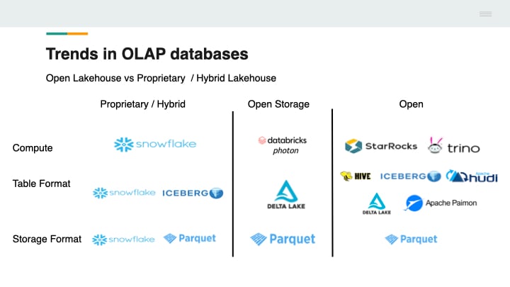
As data lakes become central to enterprise architecture, modern OLAP systems increasingly support open table formats like:
These formats enable:
-
Schema evolution
-
Partition pruning
-
Time travel and snapshot isolation
-
Interoperability across engines (e.g., Trino, Spark, StarRocks, Flink)
StarRocks, for example, supports Iceberg tables natively, allowing users to:
-
Run fast SQL queries over Iceberg without copying data
-
Join real-time Kafka streams with batch data in Iceberg
-
Apply materialized views to federated Iceberg sources
This is a big shift: rather than forcing users into proprietary storage layers, OLAP engines are becoming query engines over open lakehouse architectures.
What These Trends Mean for Architects
Modern OLAP systems:
-
Scale elastically in cloud-native environments
-
Support real-time ingestion from event streams
-
Query open data formats directly on data lakes
-
Run fast vectorized queries across billions of rows
-
Decouple compute and storage for cost efficiency
Systems like StarRocks are at the forefront of these changes — bridging traditional OLAP speed with lakehouse flexibility, and enabling organizations to move from batch BI to real-time, self-service analytics at scale.
FAQ: OLAP Systems and Modern Analytics Architecture
What exactly is the difference between OLAP and OLTP?
OLTP systems are designed to process high volumes of short transactions, such as inserting a new order or updating a user profile. These systems focus on data integrity, concurrency, and low-latency writes.
OLAP systems are designed to analyze large volumes of historical data, focusing on complex read queries, aggregations, and multidimensional exploration. They are optimized for query throughput and analytical flexibility, not transactional workloads.
Why can’t I just use my OLTP database for analytics?
You technically can, but it’s a bad idea at scale. Here's why:
-
OLTP databases are row-oriented, making large scans slow.
-
Analytical queries with multi-table JOINs and GROUP BYs are resource-intensive and may block transactional users.
-
OLTP schemas are highly normalized, which makes exploratory analysis painful.
For example: running a 10-table JOIN with aggregations over 100 million rows in PostgreSQL will likely spike memory and I/O, and result in a slow query that locks rows needed by your app.
Are OLAP systems just big relational databases?
Not quite. While some OLAP engines use SQL and relational principles (tables, schemas, JOINs), they’re architecturally different:
-
They use columnar storage, not rows
-
They apply vectorized execution for batch-style processing
-
They often use distributed, MPP (massively parallel processing) models
-
Many support materialized views, bitmap indexes, and caching at a much deeper level than general-purpose RDBMSs
In short: OLAP engines are designed from the ground up for analytical throughput.
What’s the benefit of columnar storage?
Columnar storage lets the system:
-
Read only the necessary columns for a query (unlike row stores that load full rows)
-
Compress data more efficiently (similar values in columns compress better)
-
Optimize memory and cache usage for vectorized execution
This results in much faster scans and aggregations, especially on wide tables with hundreds of columns (but where each query only touches 5–10 of them).
What is vectorized execution and why does it matter?
Traditional (row-based) execution processes one row at a time. Vectorized execution processes data in batches (vectors) — typically 1,024 values at once.
This allows:
-
Better CPU utilization via SIMD (single instruction, multiple data)
-
Fewer function calls, less overhead
-
More predictable memory access patterns, which speeds up scans
Engines like StarRocks and ClickHouse rely heavily on vectorization to reach sub-second query latencies.
Is OLAP only for batch data, or can it handle streaming data too?
Historically, OLAP was batch-only. But modern OLAP engines increasingly support streaming ingestion through Kafka, Flink, or CDC (Change Data Capture) tools.
StarRocks, for example, can:
-
Ingest data continuously via Kafka connectors
-
Use primary key tables to apply upserts
-
Automatically update materialized views on new data arrival
This enables near-real-time dashboards without needing a separate streaming analytics system.
Do I need to denormalize my data for OLAP?
Not necessarily. Older OLAP engines struggled with JOINs, so denormalization was common. But modern engines like StarRocks:
-
Handle large fact-dimension JOINs efficiently
-
Support colocate JOINs and bucket shuffle JOINs
-
Allow normalized schemas to coexist with materialized views
So, you can keep your data normalized and still get fast performance — or selectively denormalize where it improves performance or simplifies queries.
How do OLAP systems stay fast on remote object storage (like S3)?
They optimize around the weaknesses of remote storage:
-
Columnar formats reduce I/O
-
Predicate pushdown and partition pruning minimize what’s read
-
Caching and prefetching keep hot data local
-
Materialized views can be used to avoid repeated expensive scans
StarRocks, for instance, supports object storage in its shared-data mode and still delivers sub-second performance for interactive queries.
What’s the difference between a materialized view and a cube?
Materialized views are SQL-defined query results that are physically stored and periodically refreshed. They’re flexible and can be incremental.
Cubes are more rigid, pre-aggregated multidimensional arrays, often built with OLAP modeling tools. They require fixed dimensions and hierarchies.
Modern OLAP systems like StarRocks have moved toward materialized views, which are easier to manage and better suited for dynamic schemas and ad hoc analysis.
How do OLAP systems fit into a lakehouse architecture?
Lakehouses combine the flexibility of data lakes with some of the performance and structure of warehouses.
Modern OLAP systems like StarRocks integrate directly with open table formats like:
-
Apache Iceberg
-
Delta Lake
-
Apache Hudi
This allows:
-
Running fast queries directly on data lake tables
-
Combining real-time and historical data in one system
-
Avoiding data duplication between lake and warehouse
It’s a key trend: OLAP engines are becoming lakehouse-native query engines.
What’s the best way to model data for OLAP?
Start with a star schema:
-
One central fact table (e.g.,
sales,events,pageviews) -
Multiple dimension tables (e.g.,
product,customer,region,date)
Best practices:
-
Use surrogate keys (integers) for dimensions
-
Partition fact tables by time or tenant ID
-
Use materialized views for frequently queried aggregates
-
Avoid unnecessary denormalization unless JOINs are a bottleneck
StarRocks, ClickHouse, and Druid all work well with star/snowflake schemas, but StarRocks is especially JOIN-friendly at scale.
.jpg)
-1.webp)