What are SQL joins?
SQL joins are a cornerstone of relational databases. They allow us to combine data from multiple tables based on logical relationships, typically defined by foreign keys. Whether you're writing ad-hoc queries, building dashboards, or designing data pipelines, understanding joins is essential for writing efficient, correct SQL — especially when working with large datasets or distributed query engines like StarRocks, Trino, or BigQuery.
Let’s walk through the different types of joins, how they are executed under the hood, and how modern systems optimize join strategies for performance and scalability.
What Are the Different Types of Joins in SQL?
To understand how SQL joins work, let’s start with two commonly used example tables: one listing employees, and another tracking their salaries.
Table 1: Employees
| employee_id |
name |
department_id |
manager_id |
| 1 |
John Doe |
101 |
3 |
| 2 |
Jane Smith |
102 |
3 |
| 3 |
Alice Johnson |
103 |
1 |
| 4 |
Chris Lee |
101 |
2 |
| 5 |
Bob Brown |
104 |
1 |
Table 2: Salaries
| employee_id |
salary |
| 1 |
50000 |
| 2 |
60000 |
| 3 |
55000 |
| 4 |
58000 |
| 6 |
62000 |
We’ll use these two tables to demonstrate each join type in SQL and examine what kind of results they produce.
The Inner Join returns rows when there is at least one match in both tables. It is the most common type of join because it allows for the combination of rows between two tables wherever there is a matching column value.
Example - This example retrieves the names and salaries of employees whose IDs are present in both the employees and salaries tables:
SELECT a.name, b.salary
FROM employees a
INNER JOIN salaries b ON a.employee_id = b.employee_id;
The query performs an Inner Join on employees and salaries using the employee_id column as the join condition. It will return rows only where there is a matching employee_id in both tables, ensuring that only employees with corresponding salary records are listed.
What Is Left Outer Join (Left Join)?
A Left Outer Join returns all rows from the left table, along with matched rows from the right table. If there is no match, the result from the right table will be NULL.
Example - Lists all employees and their salaries, including those employees who do not have a salary record:
SELECT a.name, b.salary
FROM employees a
LEFT JOIN salaries b ON a.employee_id = b.employee_id;
This query lists every employee regardless of whether they have a matching salary record in the salaries table. For employees without salary records, the salary column in the result set will show NULL.
What Is Right Outer Join (Right Join)?
The Right Join returns all rows from the right table and the matched rows from the left table. If there is no match, the result is NULL on the side of the left table.
Example - To display all salary records along with the names of the employees, including salaries that do not match any employee ID:
SELECT a.name, b.salary
FROM employees a
RIGHT JOIN salaries b ON a.employee_id = b.employee_id;
This query ensures every salary is listed along with the employee name if available. If a salary record does not have a corresponding employee record, the name field in the result will be NULL.
What Is Full Outer Join (Full Join)?
A Full Outer Join returns rows when there is a match in one of the tables. If there is no match, the result is NULL on the side of the table without a match.
Example - To combine all records from both employees and salaries, filling in NULL where there is no match on either side:
SELECT a.name, b.salary
FROM employees a
FULL OUTER JOIN salaries b ON a.employee_id = b.employee_id;
This query displays all entries from both tables. Where an employee does not have a salary record, or a salary does not have an associated employee, the result will show NULL for the missing part.
What Is Cross Join?
The Cross Join returns the Cartesian product of rows from the tables in the join. It combines each row of the first table with each row of the second table.
Example - To illustrate the combination of every possible pair of rows from the two tables, regardless of any relationship between them:
SELECT a.name, b.salary
FROM employees a
CROSS JOIN salaries b;
This query does not use a join condition. It simply multiplies each row from employees with each row from salaries, leading to every possible combination.
What Is Self Join?
A Self Join is employed to join a table to itself as if the table were two tables, temporarily renaming at least one table in the SQL statement to facilitate the join.
Example - To find relationships within the same table, such as identifying employees who are managed by other employees:
SELECT A.name AS Employee1, B.name AS Employee2
FROM employees A, employees B
WHERE A.manager_id = B.employee_id;
In this query, the employees table is joined to itself to compare each employee against each other to find matching manager-employee relationships. The result lists pairs of employees where one is the manager of the other.
What Is Semi Join?
A Semi Join is a specialized type of join that returns rows from the first table only if there is at least one matching row in the second table. Unlike Inner Join, it does not return any columns from the second table, nor does it duplicate the rows from the first table if there are multiple matches in the second table. It's particularly useful for filtering data based on the existence of a relationship in another table, without actually retrieving data from that other table.
Example - Filters employees based on the existence of corresponding salary records:
SELECT a.name
FROM employees a
WHERE EXISTS (
SELECT 1
FROM salaries b
WHERE a.employee_id = b.employee_id
);
This query uses a subquery with the EXISTS operator to check for the presence of at least one matching row in the salaries table for each row in the employees table. It returns only the names of those employees who have corresponding entries in the salaries table.
What Is ANTI Join?
An ANTI Join returns rows from the first table where there are no corresponding rows in the second table. This join is useful for identifying records in one table that do not have related records in another table, which can be particularly helpful for data validation or identifying missing entries.
Example - Lists employees who do not have salary records:
SELECT a.name
FROM employees a
WHERE NOT EXISTS (
SELECT 1
FROM salaries b
WHERE a.employee_id = b.employee_id
);
This query employs a subquery within the NOT EXISTS clause to check for the absence of matching rows in the salaries table. It returns the names of employees who do not have corresponding salary entries, effectively performing an exclusion filter.
What are JOIN Algorithms?
When you write a SQL query that includes a JOIN, you're describing what result you want—but not how to compute it. That job falls to the database engine, which selects a join algorithm to determine how rows from different tables are matched and combined based on the join condition (usually an equality comparison on a shared key).
Join algorithms are foundational to query performance. They define the mechanics of data access, comparison, and row combination—often at a low level that you don’t see unless you dig into execution plans. But understanding how they work is critical, especially when dealing with large tables or distributed systems, because the wrong algorithm can turn a 100ms query into a multi-minute one.
Why Join Algorithms Matter
Imagine trying to join a table with 10 million rows to another with 5 million. There are many ways to do this:
-
Should we scan every row in both tables and compare all combinations (brute force)?
-
Should we pre-sort the tables and scan them in sync?
-
Should we build a hash table on one side to accelerate lookup?
Each approach has trade-offs. Some are faster but use more memory. Others are slower but more general-purpose. Which one gets used depends on many factors:
-
Data size: Is one table tiny and the other huge, or are both large?
-
Index availability: Is the join column indexed?
-
Sort order: Are either of the inputs already sorted on the join key?
-
Memory constraints: Can we afford to load a table into memory?
-
Execution environment: Are we on a single machine, or a distributed system like StarRocks or Spark?
Understanding these variables helps you design queries—and sometimes tables—that are more optimizer-friendly and more efficient at runtime.
Let’s now break down the main types of join algorithms: Hash Join, Nested Loop Join, and Merge (Sort-Merge) Join. We’ll also examine how modern query engines make decisions about which one to use in different situations.
What Is Hash Join?
The hash join is the workhorse of modern analytical databases, especially in columnar systems and MPP (Massively Parallel Processing) environments. It's designed for equi-joins (e.g., a.key = b.key) and works well when one table is significantly smaller than the other.
How It Works
-
Build Phase
The database picks the smaller of the two input tables (called the build side) and loads it into memory, creating a hash table keyed by the join column.
-
Probe Phase
It then scans the larger table (called the probe side), applies the same hash function to the join column, and looks for matches in the hash table.
-
Optional: Partitioning
If the build side is too large to fit in memory, it may be partitioned into smaller chunks, potentially spilling to disk—this is known as a grace hash join.
Visualization
Think of it like scanning a phone book (build side), storing names by first letter, and then rapidly checking an incoming list (probe side) to find matches in the correct letter bucket.
Performance Notes
-
Fast for large joins, assuming the build side fits in memory.
-
Insensitive to sort order (unlike merge joins).
-
Used heavily in data warehouses (e.g., joining small dimension tables to large fact tables).
-
Not ideal for non-equi joins (e.g., <, >).
Real-World Usage
Hash joins power many warehouse-style queries like:
SELECT f.order_id, d.region
FROM fact_sales f
JOIN dim_store d ON f.store_id = d.store_id;
Here, dim_store is small and becomes the build side, while fact_sales is scanned and matched against the hash buckets.
What Is Nested Loop Join?
The nested loop join is the simplest algorithm—conceptually and operationally. It checks every possible combination of rows, making it brute-force but flexible.
How It Works
-
For each row in the outer table:
-
Scan every row in the inner table.
-
For each pair, evaluate the join condition.
-
If the condition matches, return the combined row.
This is often how you would implement a join manually in code if you didn’t know better.
Optimizations
-
When the inner table has an index on the join column, this becomes an Index Nested Loop Join, dramatically reducing scan time.
-
If the outer table is filtered heavily, the number of loop iterations shrinks, making it viable even for larger data.
Best Used When
-
One table is small (or highly filtered).
-
No suitable hash or sort order is available.
-
Joins are non-equi (e.g., range joins like a.created_at < b.cutoff).
Real-World Usage
Nested loops are common in OLTP systems:
SELECT u.name, o.order_id
FROM users u
JOIN orders o ON u.user_id = o.user_id
WHERE u.status = 'active';
If users is filtered down to a handful of rows, the system may use a nested loop join—even if orders has millions of rows.
Performance Trade-Offs
-
Very flexible (supports any condition), but
-
O(n²) worst-case complexity for full scans.
-
Depends heavily on indexes or small row counts.
What Is Merge Join (Sort-Merge Join)?
The merge join is ideal when both input tables are already sorted by the join key. It’s highly efficient because it can walk both inputs in lockstep—like zipping two ordered lists.
How It Works
-
Sort both tables by the join key (if not already sorted).
-
Start from the beginning of both.
-
Compare keys:
-
If equal, emit a match and advance both.
-
If not, advance the lower-key row.
-
Repeat until both tables are exhausted.
Visualization
Think of it like merging two sorted Excel sheets: you scroll down both sheets at the same time and compare values as you go.
When It Shines
Drawbacks
-
Sorting is expensive if not already in place.
-
Only works for equi-joins.
-
Not suited for hash-based partitioned data in distributed systems unless a sort phase is introduced.
Use Case
SELECT a.id, b.name
FROM orders a
JOIN customers b ON a.customer_id = b.customer_id
ORDER BY a.customer_id;
If both tables are already indexed by customer_id, a merge join is ideal.
Summary: Choosing the Right Join Algorithm
| Join Type |
Best When... |
Memory Use |
Handles Sort? |
Flexibility |
| Hash Join |
One table is small, large fact/dim joins |
Medium-High |
Not required |
Only equality joins |
| Nested Loop Join |
Tables are small, or filtered, or range joins used |
Low (unless indexed) |
Not required |
Any join condition |
| Merge Join |
Both tables are sorted or indexed |
Low-Medium |
Required |
Equality joins only |
In practice, modern engines (like StarRocks, PostgreSQL, or Spark SQL) choose join algorithms automatically based on cost-based optimization (CBO) and runtime statistics. But knowing how they work helps you write queries that play to the engine’s strengths—and avoid accidentally triggering expensive plans.
Want to go deeper? We can next explore distributed join strategies like broadcast joins, shuffle joins, and colocate joins — especially relevant when working in MPP systems like StarRocks or BigQuery.
Join Strategies: Local Joins vs. Distributed Joins
In SQL, writing a JOIN is just one part of the story. The database engine must also decide how to execute that join, particularly in a distributed environment where data is partitioned across nodes. Two broad categories of execution strategies arise: local joins and distributed joins.
What are Local Joins?
In traditional, single-node databases, local joins simply refer to join operations where all relevant data resides on the same machine. Because everything is local to the same memory and disk subsystem, the join can proceed without any network transfer—making it fast and efficient.
Even in distributed databases, a join is considered “local” if the data needed for the join is co-located on the same node. In these cases, the query engine doesn’t need to reshuffle or broadcast data, and each node can independently perform its portion of the join.
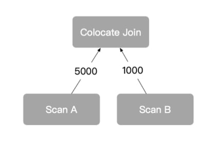
Local Joins in Distributed Systems: Co-located Joins
In distributed systems like StarRocks, the term "local join" often maps to a more specific strategy: the co-located join.
How Co-located Joins Work
-
Aligned Partitioning: Both tables are partitioned using the same hash function and key, and have the same number of buckets (partitions).
-
Node-local Execution: Since rows with matching join keys are guaranteed to be on the same node, the join can be executed locally on each node—no data movement needed.
Requirements and Considerations
-
Requires upfront coordination: The data must be bucketed or distributed based on the same join key and partition count during ingestion or table creation.
-
High performance: This is one of the most efficient join strategies, as it avoids network traffic altogether.
-
Limited flexibility: If your join keys change often or vary by workload, maintaining this co-location may be impractical.
Co-located joins are ideal for stable, repeatable workloads—e.g., joining fact and dimension tables in OLAP-style reporting systems.
What are Distributed Joins?
In a distributed database, the data needed for a join operation is typically spread across multiple nodes. Unlike local joins—where both sides of the join reside on a single machine—distributed joins require data movement to bring related rows together. This makes distributed joins more complex but also essential for scaling query processing across large datasets.
In modern MPP (Massively Parallel Processing) engines like StarRocks, Trino, and Spark SQL, distributed joins are the default strategy for handling joins across partitioned or sharded data.
Shuffling in Distributed Joins:
A key mechanism that enables distributed joins is shuffling.
-
What is shuffling?
Shuffling is the process of redistributing data across the nodes in a cluster so that rows with matching join keys from both tables end up on the same node.
-
Why is it important?
Without shuffling, the system wouldn’t be able to line up related rows. A join operation would miss matches or require inefficient data broadcasting. Shuffling is what makes parallel joins across distributed partitions possible.
-
Why does it matter for performance?
Shuffling introduces network overhead and memory pressure. The more data needs to be moved, the more expensive the operation becomes. Efficient join execution depends on minimizing how much data is shuffled—and how it's done.
Distributed Join Strategy 1: Broadcast Join
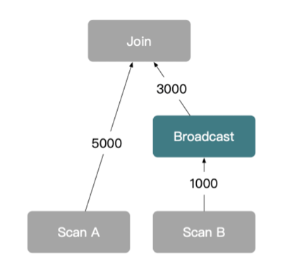
A broadcast join is a type of distributed join that avoids shuffling both tables. Instead, it replicates the smaller table to every node.
How Broadcast Joins Work
This strategy is simple and fast—when the smaller table is actually small.
Example
If you’re joining a large table of logs with a small lookup table of user roles:
SELECT logs.*, roles.role_name
FROM logs
JOIN user_roles AS roles ON logs.user_id = roles.user_id;
If user_roles is small (e.g., a few thousand rows), the engine may broadcast it.
Considerations
-
Network Cost: If the cluster has 3 nodes and the table being broadcasted has 10,000 rows, those 10,000 rows are copied to each node—resulting in 30,000 rows of network traffic.
-
Memory Limitations: The broadcasted table must fit into the memory of each worker. If it doesn’t, the join can fail or degrade in performance.
-
Best suited for:
-
Small right-hand-side tables (lookup or dimension tables).
-
Relatively small clusters.
-
Situations where reshuffling large fact tables would be more expensive.
Platform Notes
Some systems like ClickHouse only support broadcast joins in distributed mode because they lack full shuffling capability. This makes understanding the memory impact of broadcasts even more critical.
Distributed Join Strategy 2: Shuffle Join
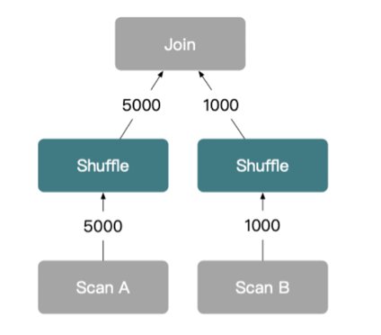
Shuffle join is a dynamic method used in distributed database systems where data from both joining tables is redistributed across all nodes based on the join key. This strategy plays a key role in enabling scalable joins across large distributed environments.
How Shuffle Joins Operate
A shuffle join (also known as a repartition join) redistributes data from both sides of the join across all nodes based on the join key.
How Shuffle Joins Work
-
Both tables are partitioned (or re-partitioned) by applying a hash function on the join key.
-
Rows are shuffled across nodes so that matching keys from both tables end up on the same node.
-
Once aligned, each node performs a local join on its data slice.
Benefits
-
Scalable: Works well for large tables with no constraints on join key size.
-
Symmetric: Neither table needs to be small; both sides can be large and evenly distributed.
-
Flexible: Useful for ad hoc queries and joins on varying keys.
Trade-Offs
-
Network Overhead: Both sides may involve heavy data movement, depending on partition size.
-
Memory Usage: Buffering for shuffling can consume significant memory if not well-tuned.
Use Cases
Shuffle joins are common in data lakehouse workloads or when querying partitioned datasets (e.g., Apache Iceberg, Hive, Delta Lake) where data is spread across nodes.
Optimized Shuffle Strategy: Bucket Shuffle Join (StarRocks)
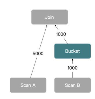
Some distributed databases, like StarRocks, implement an optimized version of shuffle joins called Bucket Shuffle Join. This strategy reduces the amount of shuffling by leveraging pre-bucketed data layouts.
How It Works
Why It Matters
-
Reduced Network Traffic: By avoiding a full reshuffle of both tables, network overhead drops significantly.
-
Improved Efficiency: Less data movement = faster query execution, especially in large clusters.
-
Automatic Optimization: StarRocks automatically detects when bucket shuffle joins are possible based on table metadata (e.g., Iceberg/Hive bucketing).
Example Use Case
Suppose sales is a large fact table bucketed on store_id, and store_info is a dimension table:
SELECT s.*, i.store_name
FROM sales s
JOIN store_info i ON s.store_id = i.store_id;
If sales is pre-bucketed on store_id, only store_info needs to be shuffled—reducing the total data movement.
When to Use Which Join Strategy
| Join Strategy |
Shuffling Required? |
Best For |
Limitation |
| Broadcast Join |
No (only replicate small table) |
Small dimension tables |
Memory-bound; poor for large right tables |
| Shuffle Join |
Yes (both sides) |
Large, unaligned datasets |
High network and memory cost |
| Bucket Shuffle Join |
Yes (one side only) |
Pre-bucketed fact/dim joins (e.g. StarRocks + Iceberg) |
Requires aligned distribution |
Distributed join strategies are essential for scalable, high-performance analytics. Whether you're designing queries for batch reporting or real-time dashboards, understanding these strategies—and how they’re executed behind the scenes—helps you anticipate bottlenecks, control costs, and design better data systems.
FAQ: SQL Joins, Algorithms, and Execution Strategies
1. What happens when a join condition is omitted?
If you omit the join condition in a regular JOIN (e.g., INNER JOIN or LEFT JOIN), the result is a Cartesian product, equivalent to a CROSS JOIN. Every row from the left table is combined with every row from the right table. This is rarely what you want for large tables and can quickly balloon to billions of rows.
2. Can you join on non-equality conditions (e.g., <, >, BETWEEN)?
Yes, but not all join algorithms support them:
-
Hash joins support only equi-joins (e.g., a.id = b.id).
-
Merge joins and nested loop joins can handle range-based or inequality joins, such as:
SELECT *
FROM events e
JOIN time_windows t ON e.timestamp BETWEEN t.start_time AND t.end_time;
However, range joins can be expensive and may default to nested loop joins unless indexes or pre-sorted data are available.
3. What’s the difference between JOIN and INNER JOIN?
They're the same. By SQL standard, JOIN defaults to INNER JOIN. This means:
SELECT * FROM A JOIN B ON A.id = B.id;
is functionally equivalent to:
SELECT * FROM A INNER JOIN B ON A.id = B.id;
4. How does a database engine choose a join algorithm?
Modern query engines use a cost-based optimizer (CBO) to decide. The optimizer analyzes:
-
Table sizes and row count estimates
-
Availability of indexes
-
Whether the inputs are sorted
-
Memory and network cost estimates
-
Distribution (single-node or multi-node)
Based on this, it selects a plan—often visible via EXPLAIN or EXPLAIN ANALYZE.
In StarRocks, for example, the optimizer may automatically select a bucket shuffle join if table metadata indicates compatible bucketing.
5. What if a join returns duplicate rows—why is that happening?
Duplicates occur when the join key matches multiple rows on either side. For example:
-- If user_id = 1 appears 3 times in orders, and once in users
-- the result will have 3 rows for that user
SELECT *
FROM users
JOIN orders ON users.user_id = orders.user_id;
To eliminate duplicates, consider using DISTINCT or aggregation, but only if semantically appropriate. Duplicates are expected in many-to-one or many-to-many joins.
6. Do indexes improve join performance in distributed systems?
Not directly.
In distributed systems like StarRocks or Trino, index-based optimizations (e.g., index nested loop joins) are not typically used, because:
-
Tables are columnar and optimized for bulk scan + vectorized processing.
-
Joins are handled using hashing or shuffling, not indexed lookups.
-
Indexes are more relevant for OLTP-style systems like PostgreSQL or MySQL.
However, pre-sorting and bucketing data can play a similar role in optimizing distributed joins.
7. What’s the performance impact of joining large tables without filtering?
Joining two large tables (e.g., billions of rows each) without filters or selective predicates can:
-
Force shuffle joins, incurring heavy network traffic
-
Require large memory buffers for intermediate data
-
Overwhelm worker nodes or cause out-of-memory (OOM) errors
Best practice: Filter as early as possible. Push predicates down before the join to reduce data volume.
8. How do distributed joins handle data skew (e.g., one key is very frequent)?
Data skew (e.g., 90% of rows sharing a single join key) causes load imbalance:
To mitigate skew:
-
Use salting or key splitting to artificially break up the skewed key.
-
Use colocated joins when possible to preserve data affinity.
-
StarRocks also supports adaptive query execution, which can sometimes handle skew dynamically.
9. Is FULL OUTER JOIN supported by all distributed engines?
Not always.
-
Engines like StarRocks and Spark SQL support FULL OUTER JOIN, but it’s more complex to execute in a distributed setting because it requires tracking unmatched rows on both sides, which may reside on different nodes.
-
Some engines do not support full outer joins or simulate them using a UNION of LEFT and RIGHT joins.
Check engine-specific documentation before relying on FULL OUTER JOIN in production.
10. Can you mix join strategies in a single query?
Yes. Complex queries involving multiple joins may use different algorithms or distribution strategies per join.
For example:
SELECT ...
FROM big_fact_table f
JOIN small_dim_1 d1 ON f.key1 = d1.key
JOIN small_dim_2 d2 ON f.key2 = d2.key;
-
The optimizer may choose a broadcast join for d1
-
A shuffle join for d2 if it's slightly larger
-
And fall back to a nested loop for a correlated subquery elsewhere
This is known as a hybrid join plan, and it’s common in cost-based optimization.
Materialized views (MVs) precompute joins, so queries on top of MVs often avoid the join altogether at runtime.
In StarRocks:
-
If a join result is already materialized, the optimizer can rewrite the query to scan from the MV instead of computing the join again.
-
This drastically reduces compute time, memory use, and network I/O.
-
MVs also help with bucket shuffle joins, as the MV can be pre-bucketed on the join key.
12. What happens if the join key contains NULLs?
By SQL standard:
-
NULL = NULL is not true, so rows with NULL join keys do not match in INNER or OUTER joins.
-
In LEFT JOIN, if the left-side key is NULL, you get a row with NULLs from the right side.
-
In FULL OUTER JOIN, if both join keys are NULL, no match will occur.
To explicitly join on NULLs, you’d need to add logic like:
ON a.key = b.key OR (a.key IS NULL AND b.key IS NULL)
But this is rarely advisable due to performance complexity.


.webp)
.jpg)